Infinite-Dimensional Diffusion Policies via Inverse Kolmogorov PDEs
This post accompanies my recent work, Visuomotor Diffusion Policies via Inverse PDEs (RoboDiff). It distills two companion notes — a first-principles derivation of the backward Kolmogorov equation (BKE) in infinite dimensions, and a hands-on PushT exposition notebook — into one narrative. The claim in a sentence: for long-horizon planning, don’t diffuse points — diffuse functions.
Why point-based diffusion policies drift
A modern diffusion policy samples an action chunk \(a \in \mathbb{R}^{T_p \times d_a}\) by running a denoiser backward from Gaussian noise. That works beautifully at short horizons. But the moment you stack the horizon \(T_p\) high — the regime you actually want for long-horizon manipulation and planning — the geometry turns against you. You are denoising in \(\mathbb{R}^{N}\) with \(N = T_p \cdot d_a\), and the standard DDPM convergence bound reads
\[\|\mu_\theta - \mu_{\text{data}}\|_{\text{TV}} = O\!\left(\sqrt{N}\,\sqrt{\text{loss}}\right).\]The \(\sqrt{N}\) is the villain. Refine the temporal grid and the bound degrades. White noise \(\mathcal{N}(0, I)\) treats every timestep as an independent coordinate, so the sampler has no notion that a trajectory should be smooth in time. The result is the familiar long-horizon drift.
The fix is not a better network. It is a better space.
The move: diffuse in a Hilbert space
Instead of an action chunk being a vector, treat it as an element of the function space
\[\mathcal{H} = L^2\!\left([0,T],\, \mathbb{R}^{d_a}\right),\]the square-integrable action trajectories. This is infinite-dimensional from the start — there is no grid to explode. The whole machinery of diffusion (a forward noising process, a score, a reverse SDE) lifts to \(\mathcal{H}\), but three objects have to be built with care: the noise, the loss, and the PDE the denoiser learns.
Noise must be colored — and the color is forced on us
On \(\mathcal{H}\) you cannot use white noise: \(\mathcal{N}(0,I)\) has no meaning when \(I\) is not trace-class. The admissible noise is a \(\mathcal{C}\)-Wiener process, driven by a covariance operator \(\mathcal{C}_\mu\) whose Mercer spectrum \(\{(\lambda_k, e_k)\}\) must be summable:
\[W_t^{\mathcal{C}} = \sum_{k=1}^\infty \sqrt{\lambda_k}\,\beta_k(t)\,e_k, \qquad \operatorname{Tr}(\mathcal{C}_\mu) = \sum_{k=1}^\infty \lambda_k < \infty.\]Each mode \(e_k\) is excited independently at rate \(\sqrt{\lambda_k}\), and the trace-class condition \(\sum_k \lambda_k < \infty\) is exactly what keeps sample paths inside \(\mathcal{H}\). In practice \(\mathcal{C}_\mu\) is a Matérn-3/2 temporal kernel; its eigenvalues decay like \(\lambda_k \sim k^{-3}\), so the noise it injects is temporally smooth by construction.
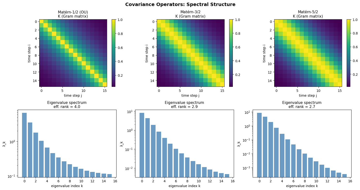 Candidate covariance kernels (Matérn-3/2, RBF, Brownian) and their eigenvalue decay
\(\lambda_k\). Smooth kernels concentrate energy in a few low-\(k\) modes — the spectral prior
that a good trajectory should be smooth.
Candidate covariance kernels (Matérn-3/2, RBF, Brownian) and their eigenvalue decay
\(\lambda_k\). Smooth kernels concentrate energy in a few low-\(k\) modes — the spectral prior
that a good trajectory should be smooth.
Sampling \(\eta = L\xi\) with \(\xi \sim \mathcal{N}(0,I)\) and \(\mathcal{C}_\mu = LL^\top\) turns white noise into colored noise. The visual difference is the whole point:
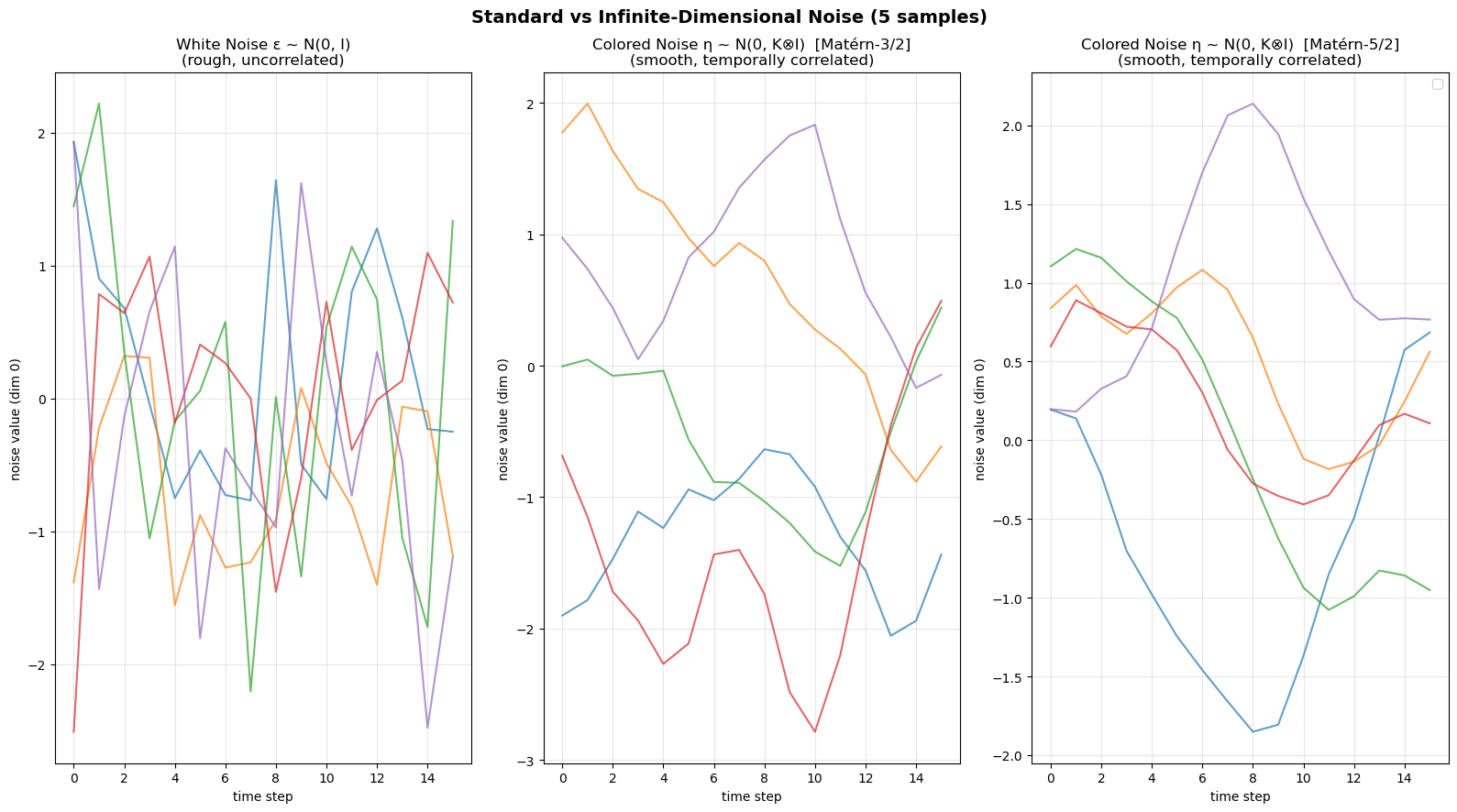 White noise (left) is jagged and coordinate-wise independent; colored noise
\(\eta \sim \mathcal{N}(0, \mathcal{C}_\mu)\) (right) is temporally coherent. Corrupting a
trajectory with colored noise perturbs it as a function, never off the manifold of
plausible motions.
White noise (left) is jagged and coordinate-wise independent; colored noise
\(\eta \sim \mathcal{N}(0, \mathcal{C}_\mu)\) (right) is temporally coherent. Corrupting a
trajectory with colored noise perturbs it as a function, never off the manifold of
plausible motions.
The Cameron-Martin space is the set of legal perturbations
Why is this the only correct noise? Because the Cameron-Martin space
\[\mathcal{H}_{\mathcal{C}} = \operatorname{Range}(\mathcal{C}_\mu^{1/2}) = \Big\{ h : \|h\|_{\mathcal{H}_\mathcal{C}}^2 = \sum_k \tfrac{\hat h_k^2}{\lambda_k} < \infty \Big\}\]is exactly the set of directions along which the Gaussian measure \(\mathcal{N}(0,\mathcal{C}_\mu)\) can be shifted while staying absolutely continuous. Push in a direction outside \(\mathcal{H}_\mathcal{C}\) — as white noise does at every reverse step — and the measures become mutually singular: the trajectory instantly leaves the support of the data. Colored noise is not a cosmetic tweak; it is a measure-theoretic necessity.
The forward process decouples spectrally
The forward dynamics are an Ornstein–Uhlenbeck (OU) SDE on \(\mathcal{H}\),
\[dX_t = -\tfrac{1}{2}X_t\,dt + dW_t^{\mathcal{C}}, \qquad X_0 \sim \mu_{\text{data}}.\]Project onto each Mercer mode \(\alpha_k(t) = \langle X_t, e_k\rangle\) and it shatters into independent scalar OU processes with a closed-form transition law,
\[d\alpha_k(t) = -\tfrac{1}{2}\alpha_k(t)\,dt + \sqrt{\lambda_k}\,d\beta_k(t), \qquad \alpha_k(t)\mid\alpha_k(0) \sim \mathcal{N}\!\big(e^{-t/2}\alpha_k(0),\ \lambda_k(1-e^{-t})\big).\]The \(\lambda_k\) prefactor on the variance is the signature of colored noise: high-energy (low-\(k\)) modes are corrupted more, high-\(k\) detail modes barely at all.
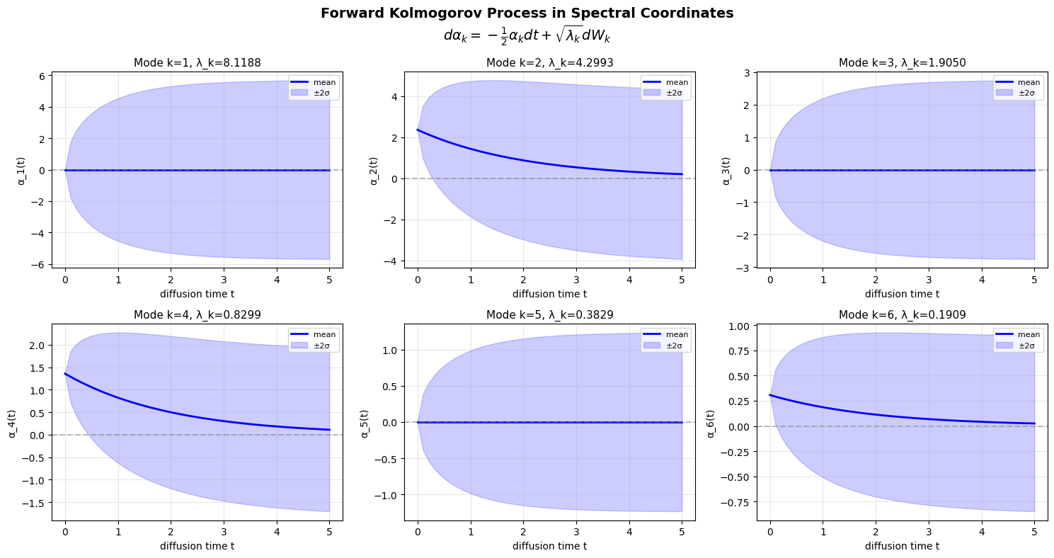 The forward process in spectral coordinates. Each mode \(\alpha_k\) mean-reverts to
\(\mathcal{N}(0,\lambda_k)\) at its own rate — an exact, per-mode Gaussian, no discretization.
The forward process in spectral coordinates. Each mode \(\alpha_k\) mean-reverts to
\(\mathcal{N}(0,\lambda_k)\) at its own rate — an exact, per-mode Gaussian, no discretization.
The star of the show: the backward Kolmogorov equation
Here is the conceptual pivot of the paper. Everything a denoiser needs to know lives in the value function
\[u(x,s) = \mathbb{E}\big[f(X_t)\mid X_s = x\big],\]and by Itô’s formula plus the martingale property, \(u\) satisfies a deterministic PDE — the backward Kolmogorov equation:
\[-\frac{\partial u}{\partial s}(x,s) = \Big\langle -\tfrac{1}{2}x,\ \nabla_x u \Big\rangle_{\mathcal{H}} + \tfrac{1}{2}\operatorname{Tr}\!\big[\mathcal{C}_\mu \cdot D^2 u\big], \qquad u(x,t) = f(x).\]This reframing is the payoff. The OU SDE describes one noisy path; to get an expectation out of it you Monte-Carlo. The BKE describes the object the denoiser actually approximates, and it does so:
- deterministically — score matching becomes structured regression against a PDE solution, not averaging over sampled rollouts;
- spectrally — in the Mercer basis the diffusion term is \(\tfrac{1}{2}\sum_k \lambda_k\,\partial^2_{e_k} u\), so modes decouple and a two-scale hierarchy (coarse locomotion vs. fine manipulation) emerges from the structure rather than being designed in;
- checkably — the score is recovered as \(\nabla_x \log p_s(x) = \mathcal{C}_\mu^{-1}\nabla_x u\), with no Lebesgue density ever needed (there isn’t one in infinite dimensions).
The training change is three lines
Everything above collapses into a tiny diff against a standard DDPM policy. The network is identical; the magic is in the noise and the loss.
- Colored noise:
η = L @ ξinstead ofε = ξ. -
Cameron-Martin loss: penalize the error in the \(\mathcal{H}_\mathcal{C}\)-norm,
\[\mathcal{L}_{\mathrm{CM}}(\theta) = \mathbb{E}\!\left[\big\|\mathcal{C}_\mu^{-1/2}\big(\eta_\theta(X_s,s) - \eta\big)\big\|_{\mathcal{H}}^2\right] = \mathbb{E}\!\left[\sum_{k=1}^\infty \frac{|\hat\eta_{\theta,k} - \hat\eta_k|^2}{\lambda_k}\right].\] - Colored reverse noise: the posterior sample
z = L @ ξ'instead ofz = ξ'.
The \(1/\lambda_k\) weighting is not a hyperparameter — it is the precision (inverse variance) of each mode. It heavily penalizes errors in low-energy modes, where the score is sharp and the denoiser must be exact, and forgives errors in high-energy modes, where the score is gentle. It is the unique weighting consistent with the Cameron-Martin geometry of \(\mathcal{N}(0,\mathcal{C}_\mu)\).
A quick sanity check that the colored forward noising is implemented correctly:
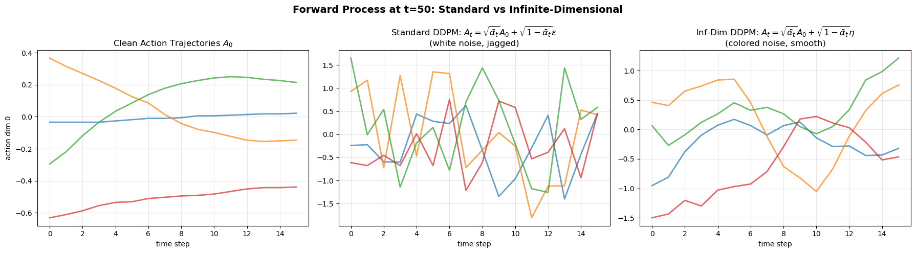 Empirical vs. analytic forward statistics: the colored forward process matches the
closed-form OU marginals mode-by-mode.
Empirical vs. analytic forward statistics: the colored forward process matches the
closed-form OU marginals mode-by-mode.
The headline result: dimension-independent convergence
Assembling Mercer → trace-class → Cameron-Martin (measure theory), the OU forward process (dynamics), and Girsanov + Pinsker (information theory) yields the paper’s main theorem.
Theorem 1 (Dimension-Independent Convergence). For a policy trained with the Cameron-Martin loss,
\[\|\mu_\theta - \mu_{\text{data}}\|_{\text{TV}} \le C_1\sqrt{\mathcal{L}_{\mathrm{CM}}(\theta)} + C_2\,e^{-T/2},\]where \(C_1\) depends only on \(\operatorname{Tr}(\mathcal{C}_\mu)\) and universal constants, and \(C_2\) only on OU-operator properties. Neither depends on the action dimension \(d_a\), the discretization resolution \(N\), nor (except exponentially) the horizon \(T\).
Contrast the two bounds side by side:
| Finite-dim DDPM | Infinite-dim (this work) | |
|---|---|---|
| Space | grid \(\mathbb{R}^N\), \(N \gg d_a\) | \(L^2([0,T],\mathbb{R}^{d_a})\), no grid |
| Noise | \(\mathcal{N}(0,I)\) (white) | \(\mathcal{N}(0,\mathcal{C}_\mu)\) (colored) |
| Loss | \(\mathbb{E}|\eta_\theta-\eta|^2\) | \(\mathbb{E}|\mathcal{C}_\mu^{-1/2}(\eta_\theta-\eta)|^2\) |
| TV bound | \(O(\sqrt{N}\sqrt{\text{loss}})\) | \(O(\sqrt{\text{loss}})\) |
The \(\sqrt{N}\) is gone. The constants collapse onto a single fixed scalar — the trace of the covariance — because the \(\mathcal{C}_\mu^{-1/2}\) weighting absorbs exactly the geometry that would otherwise leak dimension into the bound.
A physics-aware diagnostic for free
Because the true \(u\) solves the BKE exactly, you can plug the learned \(u_\theta\) back into the equation and measure the violation — the Kolmogorov residual:
\[\mathcal{R}_\theta(x,s) = \frac{\partial u_\theta}{\partial s} + \Big\langle -\tfrac{1}{2}x,\ \nabla_x u_\theta \Big\rangle_{\mathcal{H}} + \tfrac{1}{2}\operatorname{Tr}\!\big[\mathcal{C}_\mu \cdot D^2 u_\theta\big].\]This is a pointwise PDE error, not a statistical one: it needs a single query \((x,s)\) and automatic differentiation of the network — no environment rollout, no new data, no task outcome. \(\mathcal{R}_\theta \equiv 0\) iff the model solves the BKE. It is a certificate you can evaluate at inference time, which is exactly the property you want for high-stakes, robots-in-production control.
Does it actually work? Results
Theory is only worth as much as the numbers behind it. The paper validates the framework on a visuomotor manipulation benchmark and a manufacturing-flow control problem, sweeping the loss from pure MSE (\(\alpha=0\), the finite-dimensional baseline) through mixed precision to the full Cameron-Martin objective (\(\alpha=1\)).
PushT manipulation
On the PushT benchmark — align a T-shaped block with a 2-DOF pusher from pixels — the Cameron-Martin policy reaches a maximum episodic reward of ≈ 0.95 vs. ≈ 0.78 for the MSE baseline, a 17% improvement, and cuts inter-step trajectory drift by 67.6%. The gain is sharpest in the final approach phase (steps 300–400): the MSE policy develops high-frequency oscillations that destabilize contact, while the CM policy stays smooth.
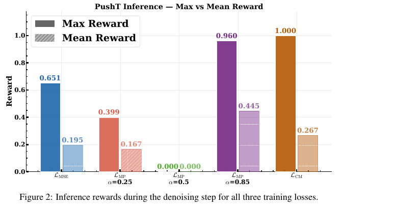 Figure 2 from the paper. Max and mean episodic reward as the loss interpolates from MSE
(\(\mathcal{L}_{\text{MSE}}\)) through mixed precision (\(\mathcal{L}_{\text{MP}}\)) to
Cameron-Martin (\(\mathcal{L}_{\text{CM}}\)). Full measure-theoretic weighting tops out at
reward 1.0.
Figure 2 from the paper. Max and mean episodic reward as the loss interpolates from MSE
(\(\mathcal{L}_{\text{MSE}}\)) through mixed precision (\(\mathcal{L}_{\text{MP}}\)) to
Cameron-Martin (\(\mathcal{L}_{\text{CM}}\)). Full measure-theoretic weighting tops out at
reward 1.0.
The Kolmogorov residual tracks this cleanly, monotonically decreasing as the precision weighting \(\alpha\) turns on:
| Loss (\(\alpha\)) | Mean residual \(\mathcal{R}\) | Reduction vs. MSE |
|---|---|---|
| MSE (\(0\)) | 0.34 | — |
| Mixed (\(0.15\)) | 0.28 | 17.6% |
| Mixed (\(0.25,\,0.50\)) | 0.22, 0.18 | — |
| Cameron-Martin (\(1.0\)) | 0.11 | 67.6% |
And the residual doubles as an oracle-free failure detector: rollouts with mean residual \(> 0.15\) correlate with task failure (max reward \(< 0.5\)), while those below \(0.10\) succeed \(> 90\%\) of the time — a real-time trustworthiness signal that needs no ground-truth reward.
Manufacturing flow (CONWIP)
The same function-space machinery transfers to a stochastic 6-station manufacturing line under CONWIP flow control, where queue dynamics are genuinely function-valued. Against an LSTM + CONWIP baseline, the infinite-dimensional policy cuts normalized work-in-process RMSE by 28.4% with high starvation-event recall (≈ 0.98).
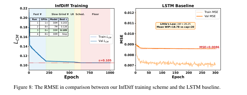 Figure 8 from the paper. Training/validation curves for the infinite-dimensional scheme
(left) vs. the LSTM baseline (right); the InfDiff floor sits at \(\varepsilon = 0.105\).
Figure 8 from the paper. Training/validation curves for the infinite-dimensional scheme
(left) vs. the LSTM baseline (right); the InfDiff floor sits at \(\varepsilon = 0.105\).
Two results stand out. First, the Kolmogorov residual localizes the bottleneck station with a 13× signal-to-noise ratio (Precision@1 = 1.0) and sub-second latency — an anomaly detector the LSTM can only infer indirectly. Second, seeding a Hamilton-Jacobi reachability computation (LevelSetPy) with the InfDiff forecast yields a certified dispatch filter that prevents 351 deadlock events across 100 runs — a 96% reduction — keeping every station above starvation and below the CONWIP cap.
Takeaways
- Diffuse functions, not points. Lifting action chunks to \(L^2([0,T])\) removes the grid whose refinement was hurting long-horizon policies.
- The color of the noise is forced. The Cameron-Martin space is the exact set of legal perturbations; colored \(\mathcal{N}(0,\mathcal{C}_\mu)\) noise is a measure-theoretic necessity, not a trick.
- Learn the PDE, not the paths. The backward Kolmogorov equation is the deterministic, spectral, checkable object the denoiser truly approximates.
- Get a theorem out of it. Cameron-Martin weighting buys dimension-independent convergence, plus a physics-aware residual you can certify at inference.
All of this costs three lines of code over a standard diffusion policy.
Read more. The full paper is here; the derivations condense two companion notes (a first-principles BKE derivation and a PushT exposition notebook). Questions and pushback welcome in the comments.