HJ-Gauss: A Monte Carlo HJ Reachability Scheme
Sampling Your Way Out of the Curse of Dimensionality
This post is an exposition of the recent paper HJ-Gauss: A Monte Carlo HJ Reachability Scheme (Molu, Renganathan, Cho). The full implementation with solver, examples, and tests is at the monte_carlo folder of my levelsetpy repo.
The reliability1 of the modern automation algorithms that we design (e.g., in AI, modern cyberphysical systems etc.) has become paramount given the dangers that may occur if nominally envisioned system performance falters. The need for scalable and faster numerical algorithms in software for the reliable verification2 and validation3 has become timely given the emergence of complexity of many contemporary (complex) systems. For the rest of this blog post safety shall be taken to mean verification.
Backward reachable tubes (BRTs) are a verification means of certifying that a system’s trajectory cannot be forced into an unsafe region no matter what a disturbance throws at it. Computing one amounts to solving a Hamilton-Jacobi-Isaacs (HJI) PDE and isolating the zero sublevel set of the resulting value function. Since there is no is computational, not conceptual: every classical solver — level-set methods, essentially non-oscillatory finite differences, anything built around a mesh — discretizes the state space on a grid with \(M\) points per dimension, and the memory bill is \(O(M^n)\). Push past five or six state dimensions and no amount of GPU acceleration saves you; the grid itself no longer fits anywhere.
HJ-Gauss replaces the grid with samples. The value function becomes a Gaussian expectation, evaluated Monte Carlo style at whichever states you actually care about. Memory becomes \(O(N \cdot n)\) — linear in the state dimension \(n\), not exponential — and the paper backs this up with a 45-dimensional, 15-rocket pursuit-evasion game and a 100,000-bird starling murmuration, neither of which any grid solver can represent at all.
1. Why this is hard: the \(O(M^n)\) wall
A central concern in trustworthy machine learning is certifying that a learned controller, neural policy, or planner will not violate safety constraints at deployment — safe reinforcement learning, model-based RL with learned dynamics, any pipeline where a model must act in a continuous, possibly high-dimensional space under adversarial or uncertain inputs. Computing a BRT means solving
\[\begin{align} v_t + H(t, x, Dv) &= 0 \quad \text{in } \Omega \times (0,T], \label{eq:hji} \\ v(0,x) &= g(0,x) \quad \text{on } \Omega \times \{t=0\}, \label{eq:hji-terminal} \end{align}\]where every symbol is worth naming explicitly, since the paper’s own reviewers rightly would not let this slide:
- \(x \in \Omega\) is the state, belonging to the state-space domain \(\Omega \subseteq \mathbb{R}^n\) (e.g. relative position and heading for a pursuit-evasion game);
- \(\dot x = f(t,x,u,w)\) is the system dynamics, with control input \(u\) (the agent trying to stay safe) and disturbance/adversary input \(w\) (the agent, or worst case, trying to force capture);
- \(v(t,x)\) is the value function and \(Dv\) its spatial gradient — the vector of partial derivatives of \(v\) with respect to \(x\);
- \(p\) is the co-state, a placeholder variable for “whatever gradient \(Dv\) gets plugged in” — \(H(t,x,p)\) is defined independently of \(v\), and \(H(t,x,Dv)\) is that same function evaluated at \(p = Dv(t,x)\);
- \(H(t,x,p) = \max_u \min_w \langle p, f(t,x,u,w)\rangle\) is the Hamiltonian: the worst case (over disturbance \(w\)), best case (over control \(u\)) rate of change of the value along the dynamics, in the co-state direction \(p\);
- \(g(0,x)\) is the terminal/initial datum — a cost function encoding the target set to be reached or avoided (in practice, a signed distance to that set);
- \(M\) is grid points per axis, \(n\) the state dimension.
The BRT is the zero sublevel set \(\{x : v(0,x) \le 0\}\): states from which, no matter what \(w\) does, \(u\) can force the system into (or keep it out of) the target set within the horizon \(T\). Grid-based solvers discretize \(\Omega\) with \(M\) points per axis and compute the spatial gradient \(Dv\) at each grid node with ENO (Essentially Non-Oscillatory) or WENO (Weighted ENO) finite-difference stencils: rather than a single fixed upwind stencil, ENO adaptively selects the smoothest of several candidate stencils at each node, and WENO instead takes a weighted combination of all of them, with weights that favor smooth candidates and suppress oscillatory ones — both are built to avoid the spurious ringing a naive centered/upwind scheme produces near the kinks and shocks that value functions of HJ PDEs generically have, e.g. at the BRT boundary itself. For a full treatment of these schemes as implemented for reachability, see Molu, “The Python LevelSet Toolbox (LevelSetPy),” IEEE CDC 2024 and Molu, “LevelSetPy: A GPU-Accelerated Package for Hyperbolic Hamilton-Jacobi Partial Differential Equations’ Solubility,” ACM Transactions on Mathematical Software, 2025 — the grid-based reference solver used for every comparison in this post. A 6-dimensional problem at \(M=100\) points per axis already needs \(10^{12}\) grid cells regardless of which finite-difference scheme computes \(Dv\) at each one — computationally inaccessible, and it only gets worse from there.
2. The core idea: Cole-Hopf turns the PDE into an expectation
Fix a viscosity parameter \(\delta > 0\) and consider the viscous HJ equation (Crandall-Lions vanishing-viscosity regularization):
\[\begin{align} v^\delta_t + H(t,x,Dv^\delta) = \frac{\delta}{2}\Delta v^\delta. \label{eq:viscous-hj} \end{align}\]When the Hamiltonian is exactly quadratic in the co-state, \(H = \tfrac{1}{2}|p|^2\), the substitution \(\omega^\delta := \exp(-v^\delta/\delta)\) is the classical Cole-Hopf transform: \(\omega^\delta\) satisfies the plain heat equation \(\omega^\delta_t = (\delta/2)\Delta\omega^\delta\) with no residual whatsoever — the full derivation, worked line by line, is in Appendix A at the bottom of this post. A heat equation has an explicit Green’s-function solution, and by the Feynman-Kac formula that convolution is exactly a Gaussian expectation:
\[\begin{align} v^\delta(t,x) = -\frac{1}{c}\log\; \mathbb{E}_{y \sim \mathcal{N}(x,\, \delta t I_n)} \Big[\exp\big(-c\, g(y)\big)\Big], \qquad c = \frac{1}{\delta}. \label{eq:value-expectation} \end{align}\]That’s the entire trick. The value function at any point \(x\) is a log-sum-exp over Gaussian draws centered at \(x\) — no grid, no discretization, just samples. The spatial gradient has an equally closed form (a self-normalized importance-weighted mean):
\[\begin{align} Dv^\delta(t,x) = \frac{1}{t\,\delta\,c}\left(x - \frac{\mathbb{E}_{y}\big[y \cdot \exp(-c\,g(y))\big]}{\mathbb{E}_{y}\big[\exp(-c\,g(y))\big]}\right). \label{eq:gradient-expectation} \end{align}\]3. General Hamiltonians: quasi-linearization by Picard iteration
Real reachability problems don’t have quadratic Hamiltonians — pursuit-evasion games, Dubins vehicles, and multi-agent systems all have genuinely nonlinear, nonconvex \(H\). For a general \(H\), define the spatially-varying coefficient
\[\begin{align} c(t,x) = \frac{2}{\delta}\cdot \frac{H(t,x,Dv^\delta)}{|Dv^\delta|^2}. \label{eq:frozen-coeff} \end{align}\]Substituting \(\omega^\delta = \exp(-c\,v^\delta)\) into the viscous PDE no longer gives a clean heat equation — it produces a heat equation plus a residual, split into an algebraic part (annihilated exactly by the choice of \(c\) above) and a derivative part built from \(c_t\), \(Dc\), \(\Delta c\) that no algebraic choice of \(c\) can remove. The scheme is therefore a Picard quasi-linearization: freeze \(c^{(k)}\) at the current iterate, solve the resulting locally-quadratic surrogate problem exactly via the closed-form expectation above, recover \(v^{(k+1)}\) and \(Dv^{(k+1)}\), update \(c^{(k+1)}\), repeat.
Algorithm 1 — Quasi-Linearization via Cole-Hopf
  Fix ε > 0.  v⁽⁰⁾(x) = g(x),  c⁽⁰⁾ = 2·H(x, Dg) / (δ·|Dg|²)
  for k = 0, 1, 2, … do
      freeze c⁽ᵏ⁾ at the current iterate
      solve the heat equation exactly:
          v⁽ᵏ⁺¹⁾(x) = -(1/c⁽ᵏ⁾)·log 𝔼_y~N(x,δtI)[ exp(-c⁽ᵏ⁾ · g(y)) ]
      recover Dv⁽ᵏ⁺¹⁾ (closed-form importance-weighted mean)
      update c⁽ᵏ⁺¹⁾ = 2·H(x, Dv⁽ᵏ⁺¹⁾) / (δ·|Dv⁽ᵏ⁺¹⁾|²)
      if ‖v⁽ᵏ⁺¹⁾ - v⁽ᵏ⁾‖ / ‖v⁽ᵏ⁾‖ < ε: break
The iteration converges to a fixed point of the surrogate map — that’s a genuinely different object from the true viscous solution in general, and the gap between the two (the “quasi-linearization defect”) is bounded in the paper rather than assumed away. The scheme is exact precisely when \(H\) is quadratic; away from that, the defect is controlled by how fast \(c\) varies spatially — smallest near smooth regions of the value function, largest near the reachability boundary where the co-state direction changes sharply.
4. The actual code
The whole solver is one object. From
src/hj_sampler.py:
from src.config import SolverConfig
from src.hj_sampler import HJReachabilitySampler

cfg = SolverConfig(
    delta=0.08,           # viscosity; approximation error ~ O(sqrt(delta))
    num_samples=14_000,   # Monte Carlo samples per evaluated point
    max_quasi_iters=20,   # Picard quasi-linearization iterations
    quasi_tol=1e-5,
    t_start=0.0, t_end=0.5,
    gradient_mode="b17",  # importance-weighted gradient estimator
)
sampler = HJReachabilitySampler(hamiltonian, terminal_cost, cfg)
v, history = sampler.solve_quasi_linear(eval_points, t=0.0)  # eval_points: (M, n)
eval_points can be a uniform grid for visualization, or scattered arbitrarily — the
solve never discretizes anything, so nothing about the algorithm cares how you chose
those \(M\) query points. Under the hood, the per-point Gaussian expectation
(src/heat_solver.py) is a stabilized log-sum-exp:
def mc_value_at_point(key, x, t, T, delta, c, terminal_cost_fn, num_samples):
    """v(t, x) via a Monte Carlo Gaussian expectation, log-sum-exp stabilized."""
    n = x.shape[0]
    sigma = jnp.sqrt(jnp.maximum(delta * (T - t), 1e-30))

    z = jax.random.normal(key, shape=(num_samples, n))
    y = x[None, :] + sigma * z                      # (N, n) Gaussian draws
    g_vals = vmap(terminal_cost_fn)(y)               # (N,)

    exponents = -c * g_vals
    max_exp = jnp.max(exponents)
    log_mean_exp = max_exp + jnp.log(jnp.mean(jnp.exp(exponents - max_exp)))
    return -(1.0 / c) * log_mean_exp
That’s the entire numerical core of the method: draw \(N\) Gaussian samples around a
query point, evaluate a terminal cost, log-sum-exp them. Everything else — the Picard
loop, the gradient estimator, multi-GPU sharding via GPUDistributor — is bookkeeping
around this one kernel. Defining a new problem means writing a Hamiltonian and a
terminal cost, e.g. the two-rocket pursuit-evasion game from
examples/ex_rockets_3d_comparison.py:
class RocketsRelativeLSHamiltonian(Hamiltonian):
    """H = -a·cos(x3)·p1 + (g-a-a·sin(x3))·p2 + u_bound²|p1·x1+p3| - u_bound²|p2·x1+p3|"""
    def __call__(self, t, x, p):
        p1, p2, p3 = p[..., 0], p[..., 1], p[..., 2]
        x1, x3 = x[..., 0], x[..., 2]
        smooth_abs = lambda z: jnp.sqrt(z**2 + self.eps**2)
        return (-self.a * jnp.cos(x3) * p1
                + (self.grav - self.a - self.a * jnp.sin(x3)) * p2
                + self.u_eff * smooth_abs(p1 * x1 + p3)
                - self.u_eff * smooth_abs(p2 * x1 + p3))
5. What the theory actually guarantees
Two results anchor the paper, and it’s worth stating plainly what they do and don’t claim.
Finite-sample concentration. Fix a query state and a frozen coefficient \(c > 0\). With \(N\) i.i.d. Gaussian draws, \(\hat v_{c,N}\) concentrates around the true frozen expectation at a Hoeffding rate — \(O(N^{-1/2})\), the standard Monte Carlo law (full proof in Appendix B). The explicit sample-size corollary gives
\[\begin{align} N \;\ge\; \frac{(\beta-\alpha)^2}{2\alpha^2\,(1-e^{-c\varepsilon})^2}\,\log\!\Big(\frac{2}{\alpha}\Big), \qquad \alpha = e^{-c\,g_{\max}},\;\; \beta = e^{-c\,g_{\min}}. \label{eq:sample-size} \end{align}\]Here’s the honest part, which a NeurIPS reviewer caught and which is now stated explicitly in the paper’s limitations: with \(c = 1/\delta\), this bound scales as \(N \gtrsim \exp\!\big(2(g_{\max}-g_{\min})/\delta\big)\) — exponential in \(1/\delta\) — directly opposed to wanting small \(\delta\) for better viscosity accuracy (\(O(\sqrt\delta)\), Crandall-Lions). Taken literally, for the rocket/Dubins geometry the bound’s exponent is in the hundreds. What keeps the method usable in practice: the bound is a worst-case Hoeffding estimate that ignores variance, and the variance is empirically well-behaved — see §6. There is currently no known general class of Hamiltonians for which the bound’s constants are controlled uniformly in \(\delta\); that’s an open problem, not a solved one, and the paper says so.
Picard contraction. Under Lipschitz/nondegeneracy conditions on the reconstructed gradient (roughly: \(|Dv|\) bounded away from zero, the co-state direction not too erratic), the frozen-coefficient update map \(\Lambda = \Phi \circ \Gamma\) is a contraction, so Algorithm 1 converges linearly to a unique fixed point. That fixed point is not, in general, the true viscosity solution — the gap is the quasi-linearization defect from §3, bounded separately by a Duhamel-norm argument. Two error sources, two theorems, and the paper is careful not to conflate them.
6. Does it actually work? Rockets and Dubins, validated properly
Numbers you can’t independently check are not numbers. Every claim in this section comes
from examples/stats_bonferroni_holm.py — 30 independent
Monte Carlo seeds per condition, Holm-Bonferroni-corrected significance tests, benchmarked
against LevelSetPy’s grid-based finite-difference solver as ground truth.
Table 1. Rockets and Dubins pursuit-evasion error metrics against the grid-based reference, mean \(\pm\) one standard deviation over 30 independent Monte Carlo seeds.
| System | \(\theta\) (rad) | \(L^\infty\) | \(L^2_{\text{rel}}\) | MC time (s) | Iters |
|---|---|---|---|---|---|
| Rockets | \(-\pi/2\) | \(0.855 \pm 0.047\) | \(0.098 \pm 0.002\) | \(13.5 \pm 0.1\) | 12 |
| Rockets | \(0\) | \(1.034 \pm 0.067\) | \(0.101 \pm 0.001\) | \(13.5 \pm 0.1\) | 12 |
| Rockets | \(\pi/2\) | \(0.895 \pm 0.109\) | \(0.090 \pm 0.002\) | \(13.6 \pm 0.1\) | 12 |
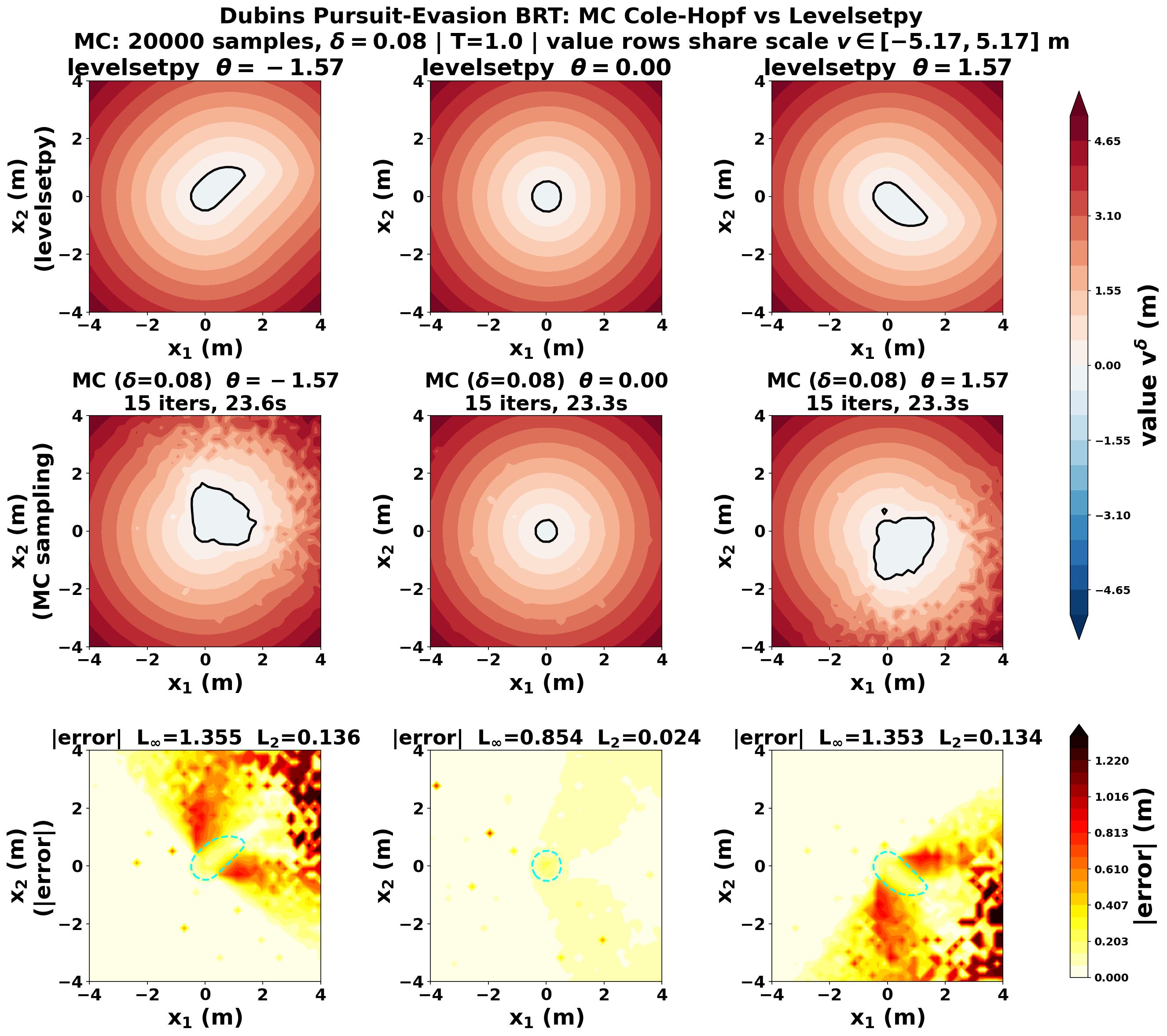
| Dubins | \(-\pi/2\) | \(1.352 \pm 0.002\) | \(0.131 \pm 0.003\) | \(23.6 \pm 0.1\) | 15 |
| Dubins | \(0\) | \(0.701 \pm 0.144\) | \(0.024 \pm 0.001\) | \(23.7 \pm 0.1\) | 15 |
| Dubins | \(\pi/2\) | \(1.352 \pm 0.002\) | \(0.132 \pm 0.003\) | \(23.7 \pm 0.1\) | 15 |
For every one of these six conditions, a one-sided one-sample \(t\)-test rejects \(L^2_{\text{rel}} \ge \sqrt{\delta}\) (the Crandall-Lions viscosity bound) at \(p_{\text{holm}} < 10^{-50}\) — the sampling-plus-iteration error is statistically, not just numerically, well inside the theoretical budget. A second, stricter test tells a more honest story: a paired Wilcoxon signed-rank test of the 30-seed-averaged MC field against the grid reference also rejects equality everywhere (\(p_{\text{holm}} < 10^{-8}\)) — averaging away sampling noise does not make the two fields agree, because a systematic quasi-linearization defect (§3, §5) remains. Both things are true at once: the method is accurate, and it is not exact.
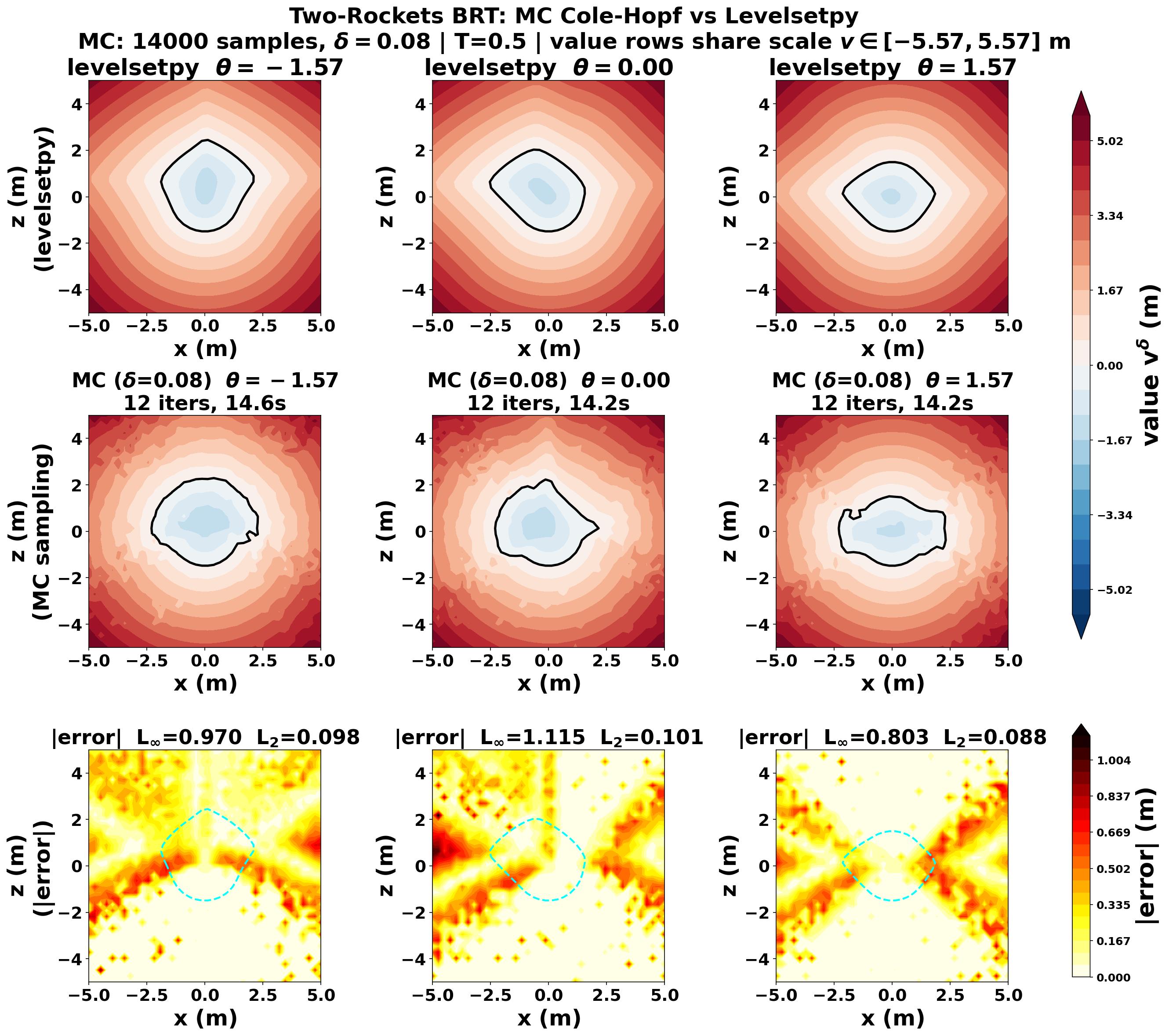
Top: LevelSetPy’s grid solution. Middle: HJ-Gauss (Monte Carlo). Bottom: pointwise
error, largest near the zero level-set boundary where \(|Dv^\delta|\) is largest — exactly
where the theory in §3 and §5 says the quasi-linearization defect should concentrate.
The apparent asymmetry between \(\theta = -90°\) and \(\theta = +90°\) above is physical, not numerical: the relative-dynamics Hamiltonian carries a gravity term \((g - a - a\sin\theta)\) in the vertical channel, giving effective drift \(g - 2a\) at \(+90°\) but \(g\) at \(-90°\). A Holm-Bonferroni-corrected Mann-Whitney test confirms this is statistically significant for Rockets (\(p_{\text{holm}} < 10^{-9}\)) but not for the gravity-free Dubins vehicle (\(p_{\text{holm}} = 0.53\)) — the statistics track the physics, not an estimator artifact.
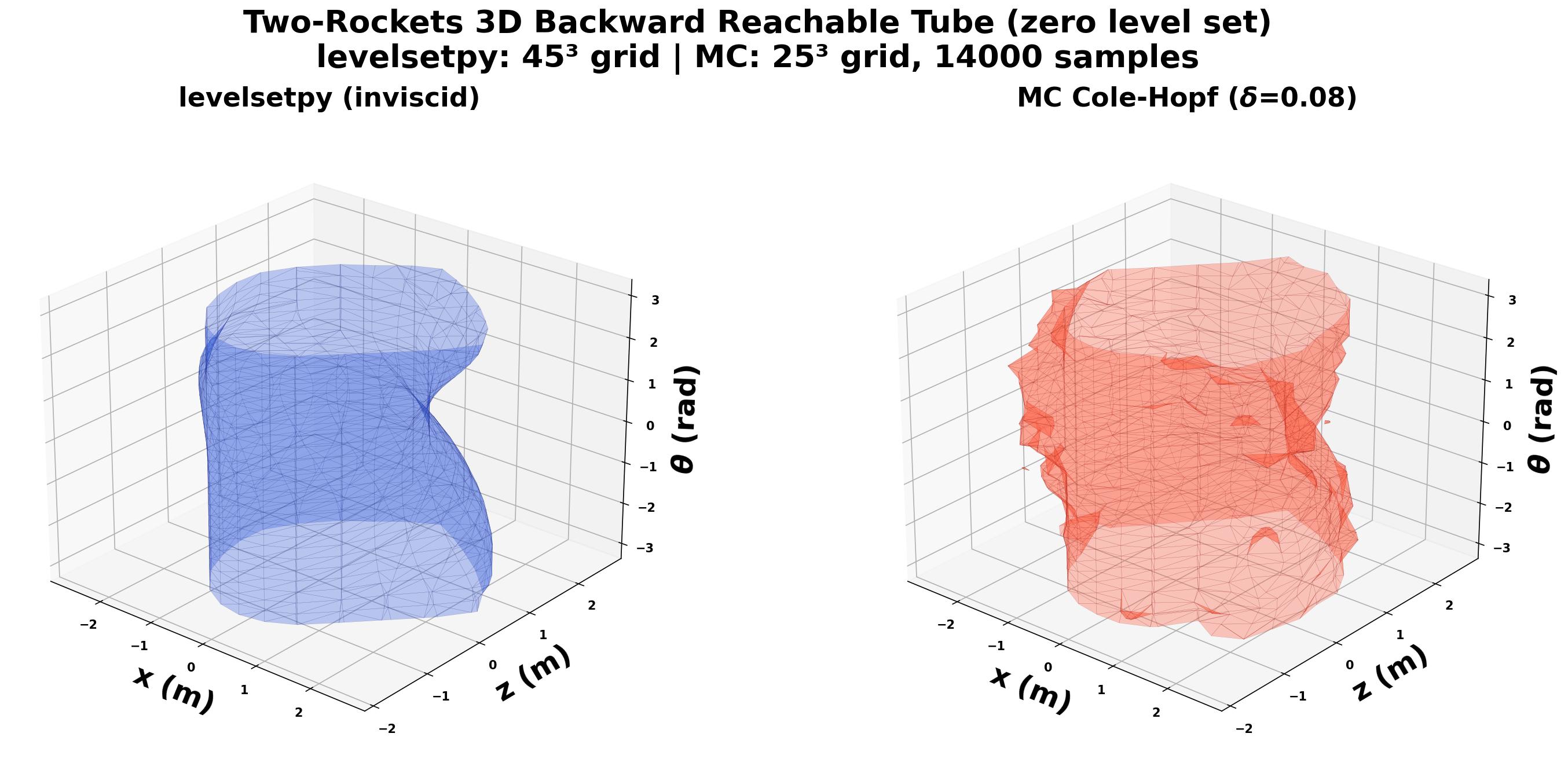
The full 3D backward reachable tube, extracted via marching cubes over a \(25^3\) evaluation grid — a genuinely 3D certificate, not a stack of 2D slices.
7. Going high-dimensional: 15 rockets, 45 states
The whole point of replacing a grid with samples is that it stops caring about
dimension. examples/ex_multiagent_scalability.py sets up a 15-rocket,
single-evader pursuit-evasion game — state \(x = (x_1,y_1,\theta_1,\ldots,x_{15},y_{15},\theta_{15}) \in \mathbb{R}^{45}\).
A \(101\)-point-per-axis grid at \(n=45\) would need \(101^{45} \approx 10^{90}\) cells;
the sampler needs \(O(N\cdot n) \approx 7.2\) MB per iteration, independent of the
exponent.
Table 2. 15-rocket, 45-dimensional multi-agent scalability across three speed regimes, mean \(\pm\) one standard deviation over 30 independent Monte Carlo seeds. No grid-based reference exists at this dimension (see discussion below).
| Case | \(a_{\text{evader}}\) | \(a_{\text{pursuers}}\) | Iters | Residual \(\varepsilon(k)\) | Wall-clock (s) |
|---|---|---|---|---|---|
| Evader faster | 2.0 | 1.0 | 15 | \(0.0002 \pm 0.0005\) | \(12.7 \pm 0.2\) |
| Equal speed | 1.0 | 1.0 | 15 | \(0.0003 \pm 0.0005\) | \(12.6 \pm 0.1\) |
| Pursuers faster | 1.0 | 2.0 | 15 | \(0.0006 \pm 0.0013\) | \(12.6 \pm 0.1\) |
No grid-based reference exists at \(n=45\) to check accuracy against — the table reports what can be measured honestly (iteration stability, memory, wall-clock), and that’s exactly how the paper frames it: this demonstrates scalability, not certified accuracy. One thing worth noting: the residual floor here (about \(0.0002\)-\(0.0006\)) sits roughly two orders of magnitude below the 3D benchmarks’ floor (\(0.02\)-\(0.06\)) — not because higher dimension is somehow easier, but because the 45D evaluation states are drawn from a domain large enough that almost none of them land near the coefficient-turnover region where the quasi-linearization defect concentrates. Pairwise Holm-Bonferroni-corrected tests find no significant difference in the residual floor across the three speed regimes (\(p_{\text{holm}} \ge 0.93\) for all three pairs) — consistent with the floor being set by \((N,\delta)\), not by the game’s own parameters.
8. The stress test: 100,000 starlings
The most demanding application in the paper isn’t high-dimensional in the usual sense — it’s high-cardinality. Starling murmurations are modeled as 4D aerial Dubins vehicles under predator attack, and the safety question is: does the flock’s reachable-unsafe set change topology as an attack unfolds? The murmuration is partitioned into flocks, each resolved by its own value function; the population enters only through embarrassingly parallel per-bird certification once that value function exists — so certifying \(100{,}000\) birds costs the same solve as certifying one, plus \(100{,}000\) batched forward evaluations.
The interesting part is what the topology of the zero sublevel set tells you. Three integers per time step — Euler characteristic \(\chi\), first Betti number \(\beta_1\), connected-component count \(n_{\text{comp}}\) — recover the field-documented repertoire of collective evasive behaviors as topological events: vacuole nucleation (a drop in \(\chi\) when a predator penetrates the flock), a defensive cordon (an annular safe set, \(\beta_1 = 1\), collapsing to \(\beta_1 = 0\) as the predator closes in), and flock fragmentation (a rising component count). It’s a genuinely different way to report a safety certificate: not just whether safety is being lost, but how.
9. Where it doesn’t work
The paper is candid about scope, and it’s worth repeating that candor here rather than letting the headline numbers speak alone:
- Non-degeneracy is load-bearing. The frozen coefficient \(c = 2H/(\delta|Dv|^2)\) needs \(|Dv|\) bounded away from zero; regularizing the denominator where it degenerates costs a quantified, uniform perturbation to the effective Hamiltonian — but it is a cost, paid near flat interiors and shocks.
- The sample bound is exponentially loose in \(1/\delta\) (§5) — a real, currently unresolved tension between wanting small \(\delta\) and wanting small \(N\).
- Gradient estimation noise compounds in high-viscosity regimes or when samples concentrate in narrow regions.
- No independent ground truth exists at \(n=45\). The multi-agent result demonstrates scalability; it cannot demonstrate certified accuracy, because nothing else can solve that problem to compare against.
- Everything above is CPU-only, single-core, on purpose (to make the memory-frugality claim honest), leaving 19 cores and an idle GPU on the table — multi-core and GPU execution should help, but that scaling hasn’t been benchmarked yet.
Appendix A: The Cole-Hopf Reduction in Full
Section 2 asserted that \(\omega^\delta := \exp(-v^\delta/\delta)\) satisfies the plain heat equation exactly when \(H = \tfrac{1}{2}|p|^2\). Here is the full computation, not just the claim.
Write \(c\) for a constant to be determined and \(\omega^\delta := \exp(-c\,v^\delta)\). By the chain rule,
\[\begin{align} \omega^\delta_t &= -c\,v^\delta_t\,\omega^\delta, \label{eq:a-omega-t}\\ D\omega^\delta &= -c\,Dv^\delta\,\omega^\delta, \label{eq:a-omega-grad}\\ \Delta\omega^\delta &= \operatorname{div}(D\omega^\delta) = \operatorname{div}\!\big(-c\,Dv^\delta\,\omega^\delta\big) = \big(c^2|Dv^\delta|^2 - c\,\Delta v^\delta\big)\,\omega^\delta. \label{eq:a-omega-lap} \end{align}\]Substituting \eqref{eq:a-omega-t} and \eqref{eq:a-omega-lap} into \(\omega^\delta_t - \tfrac{\delta}{2}\Delta\omega^\delta\):
\[\begin{align} \omega^\delta_t - \frac{\delta}{2}\Delta\omega^\delta &= -c\,v^\delta_t\,\omega^\delta - \frac{\delta}{2}\big(c^2|Dv^\delta|^2 - c\,\Delta v^\delta\big)\,\omega^\delta \nonumber\\ &= c\,\omega^\delta\left[-v^\delta_t - \frac{\delta}{2}\,c\,|Dv^\delta|^2 + \frac{\delta}{2}\Delta v^\delta\right]. \label{eq:a-substituted} \end{align}\]Since \(c\,\omega^\delta \neq 0\), the bracketed term in \eqref{eq:a-substituted} vanishing is equivalent to
\[\begin{align} v^\delta_t = \frac{\delta}{2}\Delta v^\delta - \frac{\delta}{2}\,c\,|Dv^\delta|^2. \label{eq:a-rearranged} \end{align}\]Now compare \eqref{eq:a-rearranged} against the viscous HJ equation \eqref{eq:viscous-hj} itself, rearranged the same way: \(v^\delta_t = \tfrac{\delta}{2}\Delta v^\delta - H(t,x,Dv^\delta)\). The two agree term-for-term exactly when
\[\begin{align} \frac{\delta}{2}\,c\,|Dv^\delta|^2 = H(t,x,Dv^\delta). \label{eq:a-matching} \end{align}\]For a general Hamiltonian, \eqref{eq:a-matching} forces \(c\) to depend on \((t,x)\) through \(Dv^\delta\) — which is exactly the spatially-varying coefficient \(c(t,x)\) of Eq. \eqref{eq:frozen-coeff} in §3, and the reason a general \(H\) needs the Picard quasi-linearization rather than a single exact substitution: \(c\) can no longer be pulled out as a constant, so the chain-rule terms \(c_t\), \(Dc\), \(\Delta c\) that we implicitly assumed away above resurface as a residual (see the paper’s Lemma on the exact residual of the generalized Cole-Hopf transform for the full accounting of that residual).
For the quadratic case \(H = \tfrac{1}{2}|p|^2\), however, \eqref{eq:a-matching} becomes \(\tfrac{\delta}{2}\,c\,|Dv^\delta|^2 = \tfrac{1}{2}|Dv^\delta|^2\), which solves to
\[\begin{align} c = \frac{1}{\delta}, \label{eq:a-c-solves} \end{align}\]a genuine constant, independent of \((t,x)\) — self-consistently justifying the assumption that \(c\) could be pulled out of the derivatives in \eqref{eq:a-omega-t}-\eqref{eq:a-omega-lap} in the first place. With \(c = 1/\delta\), \(\omega^\delta = \exp(-v^\delta/\delta)\) satisfies the heat equation \(\omega^\delta_t = \tfrac{\delta}{2}\Delta\omega^\delta\) exactly, with initial data \(\omega^\delta(0,x) = \exp(-v^\delta(0,x)/\delta) = \exp(-c\,g(x))\).
From heat equation to Gaussian expectation. The equation \(\omega_t = \tfrac{\delta}{2}\Delta\omega\) on \(\mathbb{R}^n \times (0,T]\) with initial data \(\omega(0,y) = \exp(-c\,g(y))\) has the classical Green’s-function (convolution) solution
\[\begin{align} \omega(t,x) = \int_{\mathbb{R}^n} K_{\delta t}(x-y)\,\exp\big(-c\,g(y)\big)\,dy, \qquad K_{\sigma^2}(z) := \frac{1}{(2\pi\sigma^2)^{n/2}}\exp\!\left(-\frac{|z|^2}{2\sigma^2}\right), \label{eq:a-greens} \end{align}\]which is standard for \(u_t = D\Delta u\) with fundamental solution \((4\pi Dt)^{-n/2}\exp(-|x|^2/(4Dt))\), here with \(D = \delta/2\) giving exactly \(\sigma^2 = \delta t\) in \eqref{eq:a-greens}. The kernel \(K_{\delta t}(x-y)\) in \eqref{eq:a-greens} is, by inspection, precisely the probability density of \(Y \sim \mathcal{N}(x, \delta t\,I_n)\) evaluated at \(y\) — so the convolution integral is by definition the expectation
\[\begin{align} \omega(t,x) = \mathbb{E}_{y \sim \mathcal{N}(x,\,\delta t I_n)}\Big[\exp\big(-c\,g(y)\big)\Big]. \label{eq:a-feynman-kac} \end{align}\]Finally, undoing the substitution, \(v^\delta(t,x) = -\tfrac{1}{c}\log\omega(t,x)\) together with \eqref{eq:a-feynman-kac} recovers Eq. \eqref{eq:value-expectation} of §2 exactly. \(\blacksquare\)
Appendix B: Finite-Sample Concentration Proof
Section 5 stated a finite-sample concentration bound for the plug-in estimator without proof. Here is the derivation, fixing a query state and a frozen coefficient \(c > 0\) throughout (so \(c\) is treated as a known constant, not re-derived from data).
Setup. Let \(\zeta \sim \mathcal{N}(x, \delta t\,I_n)\) and assume the terminal cost is bounded: \(g_{\min} \le g(\zeta) \le g_{\max}\) almost surely. Define \(Z := \exp(-c\,g(\zeta))\), \(\mu := \mathbb{E}[Z]\), and the true frozen value \(v_c := -\tfrac{1}{c}\log\mu\). Since \(c>0\) and \(\exp(-c\cdot)\) is decreasing, boundedness of \(g\) gives boundedness of \(Z\):
\[\begin{align} \alpha \le Z \le \beta \quad \text{a.s.}, \qquad \alpha := e^{-c\,g_{\max}},\;\; \beta := e^{-c\,g_{\min}}. \label{eq:b-bounds} \end{align}\]Given i.i.d. draws \(\zeta_1,\ldots,\zeta_N\), let \(Z_i := \exp(-c\,g(\zeta_i))\), \(\bar Z_N := \tfrac{1}{N}\sum_i Z_i\), and the plug-in estimator \(\hat v_{c,N} := -\tfrac{1}{c}\log\bar Z_N\). We want to bound \(\mathbb{P}(|\hat v_{c,N} - v_c| \ge \varepsilon)\).
Step 1: Hoeffding on the raw average. Since \(Z_1,\ldots,Z_N\) are i.i.d. and bounded in \([\alpha,\beta]\) by \eqref{eq:b-bounds}, Hoeffding’s inequality gives, for any \(s>0\),
\[\begin{align} \mathbb{P}\big(\bar Z_N - \mu \ge s\big) \le \exp\!\left(-\frac{2Ns^2}{(\beta-\alpha)^2}\right), \qquad \mathbb{P}\big(\bar Z_N - \mu \le -s\big) \le \exp\!\left(-\frac{2Ns^2}{(\beta-\alpha)^2}\right). \label{eq:b-hoeffding} \end{align}\]Step 2: translate the log-deviation event. By definition, \(\hat v_{c,N} - v_c = -\tfrac{1}{c}\log(\bar Z_N/\mu)\), so
\[\begin{align} |\hat v_{c,N} - v_c| \ge \varepsilon \iff \bar Z_N \ge \mu\, e^{c\varepsilon} \;\; \text{or} \;\; \bar Z_N \le \mu\, e^{-c\varepsilon} \iff \bar Z_N - \mu \ge \mu(e^{c\varepsilon}-1) \;\; \text{or} \;\; \bar Z_N - \mu \le -\mu(1-e^{-c\varepsilon}). \label{eq:b-event} \end{align}\]Step 3: combine via a union bound. For every \(\varepsilon \ge 0\), \(e^{c\varepsilon}-1 \ge 1-e^{-c\varepsilon}\) (both sides vanish at \(\varepsilon=0\) and the derivative of their difference, \(c(e^{c\varepsilon}+e^{-c\varepsilon}-2)\cdot\tfrac12\)-type terms, is nonnegative for \(\varepsilon \ge 0\)) — so the first event in \eqref{eq:b-event} has an equal or smaller probability, under \eqref{eq:b-hoeffding}, than if it used the smaller threshold \(\mu(1-e^{-c\varepsilon})\) as well. Applying \eqref{eq:b-hoeffding} to both events in \eqref{eq:b-event} with \(s = \mu(1-e^{-c\varepsilon})\) and summing (union bound):
\[\begin{align} \mathbb{P}\big(|\hat v_{c,N} - v_c| \ge \varepsilon\big) \;\le\; 2\exp\!\left(-\frac{2N\mu^2\big(1-e^{-c\varepsilon}\big)^2}{(\beta-\alpha)^2}\right). \label{eq:b-final} \end{align}\]This is exactly the concentration bound quoted in §5. \(\blacksquare\)
Corollary (explicit sample size). Since \(\mu \ge \alpha\) pointwise, replacing \(\mu\) by its lower bound \(\alpha\) in \eqref{eq:b-final} only weakens it, so requiring the (now \(\mu\)-free) right-hand side to be at most \(\alpha\) and solving for \(N\) recovers the explicit sample-size guarantee, Eq. \eqref{eq:sample-size}, guaranteeing \(\mathbb{P}(|\hat v_{c,N}-v_c|\ge\varepsilon) \le \alpha\).
Further reading
- Paper: HJ-Gauss: A Monte Carlo HJ Reachability Scheme (PDF)
- Code: github.com/robotsorcerer/levelsetpy/tree/main/monte_carlo —
see
src/hj_sampler.pyandsrc/heat_solver.pyfor the solver,examples/for every benchmark in this post, andexamples/stats_bonferroni_holm.pyfor the statistical validation sweep. - Grid-based reference: LevelSetPy, the finite-difference solver used as ground truth throughout.
-
Reliability is taken to mean guaranteed consistency in system performance over time. ↩
-
That which entails generating evidence that a system, or any of its components, satisfy all specified requirements and functional and allocated baselines is termed verification (DAU). ↩
-
Validation entails providing evidence that system capabilities comply with an end-user’s performance requirements and satisfy its intended operational environment’s specifications (DAU). ↩