 Lekan Molu
Control Commons
Intro
Here are a few control theorems, concepts and diagrams that I think every control student should know. I keep updating this post, so please check back from time to time.
Definitions, Theorems, Lemmas and such.
Nonlinear Control Theory
- A differential equation of the form
\begin{align} dx/dt = f(x, u(t), t), \quad -\infty < t < +\infty \label{eq:diff_eq} \end{align}
is said to be free (or unforced) if \(u(t) \equiv 0\) for all \(t\). That is \eqref{eq:diff_eq} becomes
\begin{align} dx/dt = f(x, t), \quad -\infty < t < +\infty \label{eq:unforced} \end{align}
- If the differential equation in \eqref{eq:diff_eq} does not have an explicit dependence on time, but has an implicit dependence on time, through \(u(t)\), then the system is said to be stationary. In other words, a dynamic system is stationary if
\begin{align} f(x, u(t), t) \equiv f(x, u(t)) \label{eq:stationary} \end{align}
- A stationary system \eqref{eq:stationary} that is free is said to be invariant under time translation, i.e.
\begin{align} \Phi(t; x_0, t_0) = \Phi(t + \tau; x_0, t_0 + \tau) \label{eq:free_stat} \end{align} - \(\Phi(t; x_0, t_0)\) is the analytical solution to \eqref{eq:diff_eq}; it is generally interpreted as the solution of \eqref{eq:diff_eq}, with fixed \(u(t)\), going through state \(x_0\) at time \(t_0\) and observed at time \(t\) later on. This is a clearer way of representing the d.e.’s solution as against \(x(t)\), which is popularly used in most text nowadays.
-
\(\Phi(\cdot)\) is generally referred to the transition function, since it relates the transformation from \(x(t_0)\) to \(x(t)\).
-
For a physical system, \(\Phi\) has to be continuous in all of its arguments. .
-
If the rate of change \(dE(x)/dx\) of an isolated physical system is negative for every possible state x, except for a single equilibrium state \(x_e\), then the energy will continually decrease until it finally assumes its minimum value \(E(x)\).
- The first method of Lyapunov deals with questions of stability using an explicit representation of the solutions of a differential equation
- Note that the second method is more of a historical misnomer, perhaps more accurately described as a philosophical point of view rather than a systematic method. Successful application requires the user’s ingenuity.
-
In contrast to popular belief that the energy of a system and a Lyapunov function are the same, they are not the same. Why? Because the Lyapunov function, \(V(x)\), is not unique. To quote Kalman, “a system whose energy \(E\) decreases on the average, but not necessarily at each instant, is stable but \(E\) is not necessarily a Lyapunov function.”
-
Lyapunov analysis and optimization: Suppose a performance index is defined to be the error criterion between a measured and an estimated signal; suppose further that this criterion is integrated w.r.t time, then the performance index is actually a Lyapunov function – provided that the error is not identically zero along any trajectory of the system.
-
Existence, uniqueness, and continuity theorem:
Let \(f(x, t)\) be continuous in \(x,t\), and satisfy a Lipschitz condition in some region about any state \(x_0\) passing through time \(t_0\):
\begin{align} R(x_0, t_0) &= ||x - x_0|| \le b(x_0) \nonumber \end{align}
\begin{align} R(x_0, t_0) &= ||t - t_0|| \le c(t_0) \quad (b, c) > 0 \end{align}
with the Lipschitz condition satisfied for \((x,t), (y,t)\) \(\in\) \(R(x_0, t_0)\), then it follows that \begin{align} ||f(x,t) - f(y,t)|| \le k \, ||x-y|| \nonumber \end{align}
where \(k>0\) depends on \(b, c\). THUS,
-
there exists a unique solution \(\Phi(t; x_0, t_0)\) of \(dx/dt\), that starts as \(x_0, t_0\) for all \(|t - t_0| \le a(t_0)\),
-
\(a(t_0) \ge \text{ Min (}{c(t_0), b(x(t_0))/M(x_0, t_0)}\), where \(M(x_0, t_0)\) is the maximum assumed by the continuous function \(f(x,t)\) in the closed, bounded set \(R(x_0, t_0)\)
-
in some small neighborhood of \(x_0, t_0\), the solution is continuous in its arguments
Observe that the Lipschitz condition only implies continuity of \(f\) in \(x\) but not necessarily in \(t\); as it is implied by the bounded derivatives in \(x\). Note that the local lipschitz condition required by the theorem only implies desired properties of a solution near \(x_0, t_0\).
The finite escape time (that is the solution leaves any compact set within a finite time) quandary does not allow us to make conclusions surrounding arbitrarily large values of \(t\). The phrase “finite escape time” describes the concept that a trajectory escapes to infinity at a finite time. In order that a differential equation accurately represent a physical system, the possibility of finite escape time has to be mitigated by an explicit assumption to the contrary. If the Lipschitz condition holds for \(f\) everywhere, then there can be no finite escape time. The proof is easy by integrating both sides of \eqref{eq:diff_eq} and using
\begin{align} \Phi(t; x_0, t_0) \le ||x_0|| + || \int_{t_0}^{t}f(\Phi(\tau; x_0, t_0), \tau)d\tau || \end{align}
\begin{align} ||x_0|| + k \int_{t_0}^{t}f(\Phi(\tau; x_0, t_0), \tau)d\tau \end{align}
where \(f(\cdot)\) obeys the lipschitz condition,
\begin{align} ||f(x,t) - f(y,t)|| \le k \, ||x-y||. \nonumber \end{align}
By the Gronwall-Bellman lemma,
\begin{align} ||\Phi(t; x_0, t_0) || \le [\exp \, k (t - t_0)] ||x_0 || \nonumber \end{align}
which is less than \(\infty \) for any finite \((t - t_0)\).
Stability
My definitions follow from R.E Kalman’s 1960 seminal paper since they are clearer to understand compared to the myriad of definitions that exist in many texts today. Stability concerns the deviation about some fixed motion. So, we will be considering the deviations from the equilibrium state \(x_e\) of a free dynamic system.
Simply put, here is how Kalman defines stability, if \eqref{eq:diff_eq} is slightly perturbed from its equilibrium state at the origin, all subsequent motions remain in a correspondingly small neighborhood of the origin. Harmonic oscillators are a good example of this kind of stability. Lyapunov himself defines stability like so:
-
An equilibrium state \(x_e\) of a free dynamic system ios stable id for every real number \(\epsilon>0\), there exists a real number \(\delta(\epsilon, t_0)>0\) such that \( x_0 - x_e \le \delta \) implies
\begin{align} ||\Phi(t; x_0, t_0) - x_e|| \le \epsilon \quad \forall \quad t \ge t_0 \nonumber \end{align}
This is best imagined from the figure below:
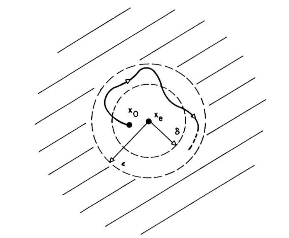
Put differently, the system trajectory can be kept arbitrarily close to the origin/equilibrioum if we start the trajectory sufficiently close to it. If there is stability at some initial time, \(t_0\), there is stability for any other initial time \(t_1\), provided that all motions are continuous in the initial state.
- Asymptotic stability: The requirement that we start sufficiently close to the origin and stay in the neighborhood of the origin is a rather limiting one in most practical engineering applications. We would want to require that our motion should return to equilibrium after any small perturbation. Thus, the classical definition of Lyapunov stability is
- an equilibrium state \(x_e\) of a free dynamic system is asymptotically stable if
- it is stable and
- every motion starting sufficiently near \(x_e\) converges to \(x_e\) as \(t \rightarrow \infty\).
- put differently, there is some real constant \(r(t_0)>0\) and to every real number \(\mu > 0\) there corresponds a real number \(T(\mu, x_0, t_0)\) such that \(||x_0 - x_e|| \le r(t_0)\) implies
\begin{align} ||\Phi(T; x_0, t_0)|| \le \mu \quad \forall \quad t \ge t_0 + T \nonumber \end{align}
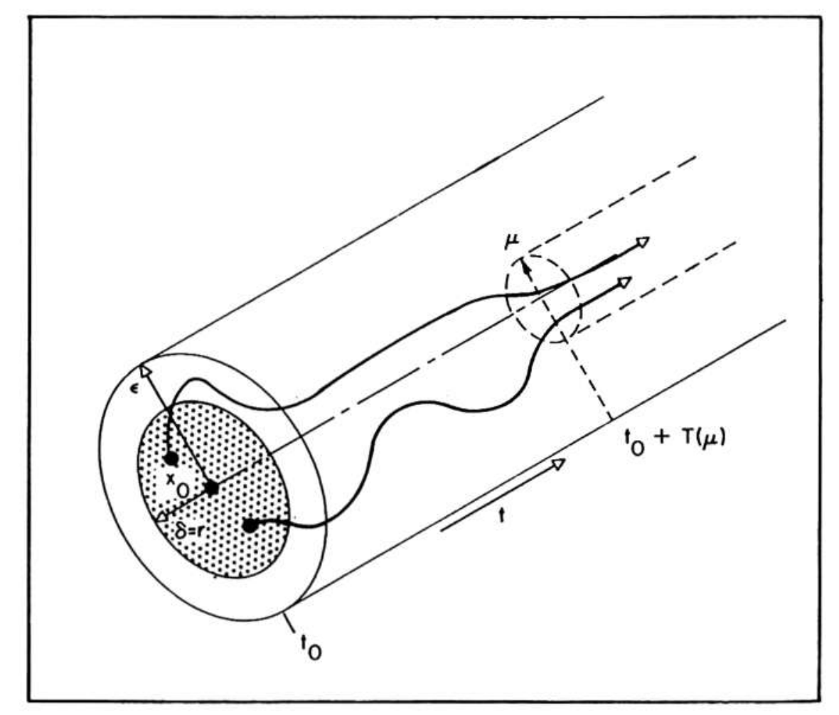 Fig. 1. Definition of asymptotic stability. Courtesy of R.E. Kalman
 - an equilibrium state \(x_e\) of a free dynamic system is asymptotically stable if
Asymptotic stability is also a local concept since we do not know aforetime how small \(r(t_0)\) should be. For motions starting at the same distance from \(x_e\), none will remain at a larger distance than \(\mu\) from \(x\) at arbitrarily large values of time. Or to use Massera’s definition:
- An equilibrium state \(x_e\) of a free dynamic system is equiasymptotically stable if
- it is stable
-
every motion starting sufficiently near \(x_e\) converges to \(x\), as \(t \rightarrow \infty\) uniformly in \(x_0\)
-
Interrelations between stability concepts: This I gleaned from Kalman’s 1960 paper on the second method of Lyapunov.
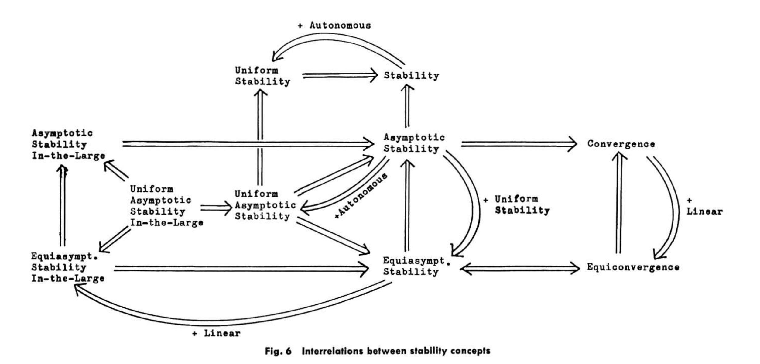 Fig. 1. Interrelations between stability concepts. Courtesy of R.E. Kalman
- For linear systems, stability is independent of the distance of the initial state from \(x_e\). Nicely defined as such:
- an equilibrium state \(x_e\) of a free dynamic system is asymptotically (equiasymptotically) stable in the large if (i) it is stable
(ii) every motion converges to \(x_e\) as \(t \rightarrow \infty \), i.e., every motion converges to \(x_e\), uniformluy in \(x_0\) for \(x_0 \le r\), where \(r\) is fixed but arbitrarily large
To be Continued