Optimal Control: Model Predictive Controllers.
</div>
Table of Notations and Abbreviations |
|||
|---|---|---|---|
| Notation | Meaning | Abbreviation | Meaning |
| $z^{-1}$ | Unit delay operator | MFD | Matrix Fraction Description |
| $x_{\rm \rightarrow}$ | Future values of x | LTI | Linear Time Invariant |
| $x_{\rm \leftarrow}$ | Past values of x | FSR | Finite Step Response |
| $\Delta = 1 - z^{-1}$ | Differencing Operator | FIR | Finite Impulse Response |
| $z^{-1}$ | Backward shift operator (z-transforms) | TFM | Transfer Function Model |
| $n_y$ | Output Prediction Horizon | SISO | Single-Input Single Output |
| $n_u$ | Input Horizon | MIMO | Multiple-Input Multiple Output |
| $u(k-i)$ | Past input | IMC | Internal Model Control |
| $y(k-i)$ | Past output | IM | Independednt Model |
###
If you are already familiar with LQ methods, you can skip this section and go straight to Model Predictive Controllers
Optimal controllers belong to the class of controllers that minimize a cost function with respect to a predicted</u> control law over a given prediction horizon</u>. They generate a desired output control</u> sequence from which the optimal _control law_</u> may be determined.
Take your car cruise speed control for an example. The vehicle dynamics of the car is _modeled_ into the cruise control system. The road curvature ahead of you gets _predicted_ online as you drive and _control sequences_ are generated based on an *internal model* (*prediction*) of the slope of the road/road curvature using past observations; other disturbances (such as rain, friction between tire and road) are modeled into the prediction ideally. At time \(k + 1\), only the first element (control action) within the generated control sequence is used as a feedback control mechanism for your car. At the next sampling time instant, new predictions are made based on the prediction horizon and a new control sequence is generated online. Again, the chosen control action is the first element in the control sequence such that we are constantly choosing the best among a host of control actions using our anticipated prediction of the road curvature and other environmental variables to give the desired performance.
</br>
Optimal controllers are mostly used in discrete processes (others have postulated continuous time models for such controllers but the vast majority of commercial users of optimal controllers are in discrete time) and are very useful for processes where the setpoint is known ahead of time. Typically, a criterion function is used to determine how well the controller is tracking a desired trajectory. An example model predictive controller (MPC) criterion function, in its basic form, is given as
<a name = eqn:cost-function></a> \begin{equation} \label{eqn:cost function} J = \sum\nolimits_{i=n_w}^{n_y} [\hat{y}(k+i) - r(k + i)]^2 \end{equation}
where \(i\) is typically taken as 1, \(n_y\) is the prediction horizon, \(\hat{y}(k+i)\) is the prediction and \(r(k+i)\) is the desired trajectory (or setpoint).
The controller output sequence, \(\Delta u \), is obtained by minimizing \(J\) over the prediction horizon, \(n_y\), with respect to \(\Delta u \), i.e.,
\begin{equation} \Delta u = \text{arg} \min_{\rm \Delta u} J \label{eqn:min J} \end{equation}
where \(\Delta u \) is the future control sequence.
</br>
If equation \eqref{eqn:cost function} is well-posed\(^{1}\), then \(\Delta u \) would be optimal with respect to the criterion function and hence eliminate offset in trajectory tracking.
</br>
It becomes obvious from equation \eqref{eqn:cost function} that minimizing the criterion function is an optimization problem. One useful approach in typical problems is to make \(J\) quadratic such that the model becomes linear; if there are no contraints, the solution to the quadratic minimization problem is analytic.
**Linear Quadratic (LQ) Controllers**
Linear Quadratic Controllers are indeed predictive controllers except for the infinite horizon which they employ in minimizing the criterion function. The criterion function is minimized only once resulting in an optimal controller output sequence from which the controller output is selected. Similar to model predictive controllers, they are in general discrete time controllers. For a linear problem such as
<a name=eqn:state-model></a> \begin{gather} \label{eqn:state-model} x(k+1) = A \, x(k) + B \, u(k) \nonumber \newline y(k) = C^T \, x(k) \nonumber \end{gather}
The cost function is typically constructed as
<a name=eqn:LQ-cost></a> \begin{equation} \label{eqn:LQ-cost} J = \sum_{k=0}^n x^T(k)\,Q\,x(k) + R \, u(k)^T \, u(k) + 2 x(k)^T \, N \, u(k) \end{equation}
where \(n\) is the terminal sampling instant, \(Q\) is a symmetric, positive semi-definite matrix that weights the \(n\)-states of the matrix. \(N\) specifies a matrix of appropriate dimensions that penalizes the cross-product between the input and state vectors, while \(R\) is a symmetric, positive defiite weighting matrix on the control vector , \(u\).
Other variants of equation \eqref{eqn:LQ-cost} exist where instead of weighting the states of the system, we instead weight the output of the system by constructing the cost function as
<a name=eqn:LQ-costy></a> \begin{equation} \label{eqn:LQ-costy} J = \sum_{k=0}^n y^T(k) \,Q \,y(k) + R\, u(k)^T \, u(k) + 2 x(k)^T \, N \, u(k) \end{equation}
In practice, it is typical to set the eigen values of the \(Q\)-matrix to one while adjusting the eigenvalue(s) of the \(R\) matrix until one obtains the desired result. \(N\) is typically set to an appropriate matrix of zeros. This is no doubt not the only way of tuning the LQ controller as fine control would most likely require weighting the eigen-values of the Q-matrix differently (this is from my experience when tuning LQ controllers).
If we model disturbances into the system’s states, the optimization problem becomes a stochastic optimization problem that must be solved. But the separation theorem applies such that we can construct a state estimator which asymptotically tracks the internal states from observed outputs using the algebraic Riccati equation given as
\begin{equation} \label{eqn:Riccati} A^T P A -(A^T P B + N)(R + B^T P B)^{-1}(B^T P A + N) + Q. \end{equation}
\(P\) is an unknown \(n \times n\) symmetric matrix and \(A\), \(B\), \(Q\), and \(R\) are known coefficient matrices as in equations \eqref{eqn:LQ-cost} and \eqref{eqn:LQ-costy}. We find an optimal control law by solving the minimization of the deterministic LQ problem, equation \eqref{eqn:LQ-cost} which we then feed into the states.
The optimal controller gains, \(K\), are determined from the equation
\begin{equation} K_{lqr} = R^{-1}(B^T \, P + N^T) \end{equation}
where \(P\) is the solution to the algebraic Riccati equation \eqref{eqn:Riccati}.
In classical control, we are accustomed to solving a control design problem by determining design parameters based on a given set of design specifications (e.g. desired overshoot, gain margin, settiling time, e.t.c). Discrete LQ controllers pose a significant difficulty with respect to solving such problems as it is challenging to solve the criterion function in terms of these design parameters since discrete state space matrices hardly translate to any physical meaning. If you use the orthogonal least squares algorithm or forward regression orthogonal least squares in identifying your physical system, you might be able to make some sense of your model though.
It turns out that if the cost function is quadratic in the parameters and the state space matrices are in continuous time, the weighting matrices would no longer correspond to the artificial, \(A\), \(B\), and \(C\) matrices (which is indeed what they are in the discrete state space).
<a name=Model-Predictive-Controllers></a> ####**
Basically, for inifinite horizon controllers such as LQ methods, this means there is no model mismatch between the predictor model and the plant. In practice, this is tough to achieve as disturbances play a large role in virtually all real-world systems. Typically in state-space or transfer function control model structures, we’ll add an integrator in the feedback loop to correct for offset errors at steady state. This would not be optimal in zeroing steady-state errors in an MPC approach. One way of avoiding mismatch is to include an integrator in the prediction model as an internal model of the disturbance. This could be a CARIMA (Controlled Auto Regressive Integral Moving Average) model, for example. A typical CARIMA model takes the polynomial form
<a name=eqn:carima></a> \begin{equation} \label{eqn:carima} A(z^{-1})\,y(k) = B(z^{-1})\,u(k) + \dfrac{C(z^{-1})}{1-z^{-1}}\,e(k) \end{equation}
where \(A\), \(B\), and \(C\) are polynomials in the backward shift operator \(z^{-1}\) given by
\begin{equation} \label{eqn:poly} A(z^{-1}) = 1 + a_1\,z^{-1} + a_2 + \, z^{-2} + \cdots + a_{n_a}z^-{n_a} \nonumber \end{equation}
\begin{equation} B(z^{-1}) = b_1 + b_2\, z^{-1} + b_3 \, z^{-2} + \cdots + b_{n_b}z^-{n_b} \nonumber \end{equation}
\begin{equation} C(z^{-1}) = c_0 + c_1\, z^{-1} + c_2 \, z^{-2} + \cdots + c_{n_b}z^-{n_c}, \end{equation}
and \(y(k)\), \(u(k)\) and \(e(k)\), for \(k = 1, 2\), \(\cdots \) are respectively the plant output, input and integrated noise term in the model.
MPC’s are generally good and better than traditional PID controllers if correctly implemented in that they handle disturbances typically well and can anticipate future disturbances thereby making the control action more effective as a result. This is because of an internal model of the plant that allows them to anticipate the future “behavior” of a plant’s output and mitigate such errors before the plant reaches the “future time”.
Rossiter gives a classic analogy in the way human beings cross a road. It is not sufficient that a road is not busy with passing cars on it. As you cross, you constantly look at ahead (your prediction horizon) to anticipate oncoming vehicles and update your movement (=control action) based on your prediction (based on past observations).
Accurate prediction over a selected horizon is critical to a successful MPC implementation.
Below are a brief overview of common models employed in MPC algorithms. Readers are referred to System Identification texts e.g., Box and Jenkins, Billings, or Ljung where data modeling and system identification methods are elucidated in details.
####
We briefly discuss the common classical models that have been accepted as a standard by the control community in the past two-some decades. Linear models obey the superposition principle. Put differently, their internal structure can be approximated by a linear function in the proximity of the desired operating point. In general, linear system identification belong in two large categories: parametric and non-parametric methods. I will only touch upon parametric methods as these are the most commonly employed models in MPC approaches.
#####
The general structure of the linear finite-horizon system can be written as
\begin{equation} \label{eqn:ARMAX} A(z^{-1})\,y(k) = \dfrac{B(z^{-1})}{F(z^{-1})}\,u(k) + \dfrac{C(z^{-1})}{D(z^{-1})}\,e(k) \end{equation}
with \(A(z^{-1}), \, B(z^{-1}), \, C(z^{-1}) \) defined as in equation \eqref{eqn:poly} and the \(F(z^{-1}), \text{ and } D(z^{-1})\) polynomials defined as
\begin{equation} D(z^{-1}) = 1 + d_1\,z^{-1} + d_2 + \, z^{-2} + \cdots + d_{n_d}z^{-n_d} \nonumber \end{equation}
\begin{equation} F(z^{-1}) = 1 + f_1\,z^{-1} + f_2 + \, z^{-2} + \cdots + f_{n_f}z^{-n_f} \end{equation}
The autoregressive part is given by the component \(A(z^{-1}) \, y(k)\), while the noise term is modeled as a moving average regression model in \(\dfrac{C(z^{-1})}{D(z^{-1})}\,e(k)\); the exogenous component is given by \(\dfrac{B(z^{-1})}{F(z^{-1})}\,u(k)\).
#####
If in equation \eqref{eqn:ARMAX}, \(B(z^{-1}) = 0\) and \(C(z^{-1}) = D(z^{-1}) = 1\) then we have an AR model,
\begin{equation} y(k) = -a_1 \, y(k-1) - a_2 \, y(k-2) - \cdots - a_{n_a} \, y(k-{n_a}) \end{equation}
Alternatively, if \(A(z^{-1}) = 1\) , \(B(z^{-1}) = 0, \, \text{ and } \, C(z^{-1}) = 1 \) then we end up with the regression
\begin{equation} y(k) = - d_1 \, y(k-1) - d_2 \, y(k-2) - \cdots - d_{n_d} y(k - n_d) + e(k) \end{equation}
#####
If \(A(z^{-1}) = 1\), \(B(z^{-1}) = 0\) and \(D(z^{-1}) = 1\), then we have the following moving average noise model
\begin{equation} y(k) = e(k)+ c_1e(k-1) + \cdots + c_{n_c}e(k-n_c) \end{equation}
#####
If \(F(z^{-1}) = 1\), and \(C(z^{-1}) = D(z^{-1}) =1\), we obtain the ARX structure
\begin{equation}
\begin{split}
y(k) & = -a_1 \, y(k-1) - \cdots - a_{n_a} \, y(k-{n_a}) + b_1u(k-1)
&+\cdots + b_{n_b}u(k-n_b) + e(k)
\end{split}
\end{equation}
#####
Setting \(B(z^{-1}) = 0\), and \(D(z^{-1}) = 1\), we obtain the ARMA model,
\begin{equation}
\begin{split}
y(k) & = -a_1 \, y(k-1) - \cdots - a_{n_a} \, y(k-{n_a}) + c_1eu(k-1)
&+\cdots + c_{n_c}e(k-n_c)
\end{split}
\end{equation}
#####
If in equation \eqref{eqn:ARMAX}, \(A(z^{-1}) = F(z^{-1}) = 1 \text{ and } C(z^{-1}) = 0\), we have an FIR model. This can be rewritten as
\begin{equation} y(k+i) = \sum_{j=0}^{n_y - 1} \, h_j\, u(k-j+i-1) \end{equation}
for predictions of the process output at \(t = k+i\) with \(i \geq 1\).
The FIR model has the advantage of being simple to construct in that no complex calculations are required of the model and model assumptions are required. They are arguably the most commonly used in commercial MPC packages. However, it does come up short for unstable systems and it also requires a lot of parameters to estimate an FIR model.
My Github repo has various examples where typical ARX, ARMAX, Impulse Response and AR models, are identified from finite data.
#####
#####
\begin{equation} y(k) = \sum_{j=0}^{n_s - 1} \, s_j\, \Delta u(k-j-1) \end{equation}
where \(\Delta\) is the differencing operator (\(\Delta = 1 - q^{-1}\)) and \(q^{-1}\) is the backward shift operator. \(n_s\) is the number of step response elements \(s_j\) used in predicting \(y\).
**Predictions in System Models**
#####
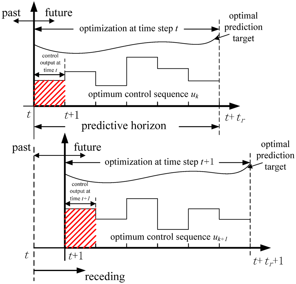
-
At a current time, \(k\), we predict an output, \(\hat{y}_k\), over a certain output horizon, \(n_y\), based on a mathematical model of the plant dynamics. The predicted output is a function of future possible control scenarios.
-
From the proposed scenarios, the strategy that delivers the best control action to bring the current process output to the setpoint is chosen.
-
The chosen control law is applied to the real process input only at the present time \(k\).
The above procedure is repeated at the next sampling instant leading to an updated control action with correctness based on latest measurements. In literature, we refer to this as the receding horizon concept
Other model-based controllers include pole-placement methods and Linear Quadratic methods. When there are no contraints on the control law and the setpoint is not complex, LQ-, pole-placement and predictive controllers generally yield an equivalent result.
We will assume the model of the plant has been correctly estimated as mentioned in the previous post. The model to be controlled (= plant) is used in predicting the process output over a defined prediction horizon, $n_y$. Typically, we would want to use an \(i\)-step ahead prediction based on our understanding of the system dynamics. The prediction horizon needs to be carefully selected such the computed optimal control law is not equivalent to a linear quadratic controller. Typically this happens when \(n_y - n_u\) is greater than the open-loop settling time and \(n_u\) is \(\geq\) 5. For large \(n_y - n_u\) and large \(n_u\), Generalized Predictive Controllers give an almost equal control to an optimal controller with the same weights. With \(n_y - n_u\) and \(n_u\) small, the resulting control law may be severely suboptimal. Model predictive controllers are implemented in discrete time since control decisions are made discretely ( = instanteneously). Continuous time systems are sampled to obtain a discrete-time equivalent. The rule of thumb is that the sampling time should be \(10 - 20\) times faster than the dominant transient response of the system (e.g. rise time or settling time).
It is important not to sample at a faster rate than the dominant transient response of the system; otherwise, the high frequency gains within the system will not be picked up by the model. In other words, we should sample fast enough to pick up disturbances, but no faster.
Model Predictive Controllers are easy to implement when the model is linear and discrete but they do find applications in nonlinear processes as well. It behooves that a nonlinear model of the process would then be employed to design the controller in such an instance. Nonlinear models will be treated in a future post. Nonlinear systems that use model predictive control tend to have a more rigorous underpinning.
Within the framework of model predictive controllers, there are several variants in literature. Among these variants are Clarke’s Generalized Predictive Controllers (GPCs), Dynamic Matrix Control, Extended Predictive Self-Adaptive Control (EPSAC), Predictive Functional Control (PFC), Ydstie’s Extended Horizon Adaptive Control (EHAC), and Unified Predictive Control (UPC) et cet’era. MPCs find applications in nonminimum phase systems, time-delay systems and unstable processes. I will briefly do a once-over on MAC, DMC and GPC with transfer function models and come back full circle to describe GPC with state-space models since these are generally straightforward to code and has less mathematical labyrinths.
####
Generally, these make use of impulse response function models. Suppose we denote the output of a discrete LTI system by a discrete impulse response \(h(j)\) as in
\begin{equation} H(z^{-1}) = A^{-1}(z^{-1}) \, B^(z^{-1}) \end{equation}
it follows that the output can be written as a function of \(h(t)\) as follows
\begin{equation} \label{eqn:impulse} y(t) = \sum_{j=1}^{n=\infty} \, h(j) \, u(t-j) \end{equation}
where \(h(j)\) are the respective coefficients of the impulse response. If we assume a stable and causal system, for an \(n\) terminal sampling instant, equation \eqref{eqn:impulse} becomes
\begin{equation} \label{eqn:impulse-lim} y(t) = \sum_{j=1}^{n} \, h(j) \, u(t-j) \end{equation}
such that we can compute the recursive form of equation \eqref{eqn:impulse-lim} as
\begin{equation} \label{eqn:impulse-rec} y_{mdl}(t + k) = \tilde{h}^T \, \tilde{u}(t + k) = \tilde{u}^T(t + k)\, \tilde{h} \end{equation}
where, \[\tilde{h}^T = h(1), \, h(2), \, h(3), \, \ldots, \, h(n) \] and \[\tilde{u}^T(t + k) = u(t + k - 1), \, u(t + k - 2), \, u(t + k -3), \, \ldots, \, u(t + k - n) \].
The cost function is given by
\begin{gather} \label{eqn:mac-cost}
J_{MAC} &= e^T \, e + \beta^2 \Delta u^T \Delta u
\end{gather}
where \(e = y_r - y_{mdl}\), and \(\beta\) is a penalty function for the input variable \(u(t)\).
- Define a reference trajectory, $y_{r}$, that $y(k)$ should track.
- Tune output predictions based on an $FIR$ model order to deal with model disturbances and uncertainties.
- Use $\beta$ to penalize the control law.
- Formulate the output predictions using equation \eqref{eqn:impulse-rec} with the assumption that the plant is stable and causal.
####
Here, a finite step response model is employed in the prediction. It is essentially composed of three tuning factors viz., the prediction horizon, \(n_y\), control weighting factor, \(\beta\), and the control horizon, \(n_u\).
- The process is stable and causal process
####
It seems to me that most literature is filled with prediction of the output described by a transfer function model. I assume this is due to their relative easiness of computation compared against FIR and FSR models and their applicability to unstable processes. Most papers out of Europe tend to favor transfer function methods while US researchers typically prefer state-space methods. Typically, Diophantine identity equations are used to form the regressor model. In my opinion, this is royally complex and more often than not obscures the detail of what is being solved. My advice is one should generally stay out of Diophantine models when possible and only use them when necessary. I will briefly expand on this treatment and focus on MPC treatments using recursive state space models when describing GPC algorithms.
The transfer function model is of the form:
\begin{equation} \label{eqn:tf_model} y(k) = \dfrac{z^{-d}B(z^{-1})}{A(z^{-1})}u(k-1) \end{equation}
with \(A(z^{-1})\) and \(B(z^{-1})\) defined by the polynomial expansions. A close inspection of equation \eqref{eqn:tf_model} reveals that the transfer function model subsumes both the FIR (i.e. \(A\) = 1 and the coefficients of the \(B\) polynomial are the impulse response elements) and FSR models (i.e. A = 1 and the coeeficients of the \(B\) polynomial are the step response coefficients \(b_0 = s_0; \, b_j = s_j - s_{j-1} \forall j \geq 1 \).
Transfer function models have the good properties of using greedy polynomial orders and variables in representing linear processes but an assumption about the model order has to be made.
#####
Another way of writing equation \eqref{eqn:tf_model} is by forming an \(i\)-step ahead predictor as follows:
\begin{equation} \label{eqn:tf_isa} y(k + i) = \dfrac{z^{-d}B(z^{-1})}{A(z^{-1})}u(k + i -1) \end{equation}
It follows from the certainty equivalence principle that if we substitute the delay, \(d, \text{ and } B, \, A \) polynomials with their estimates (i.e. \(\hat{d}, \hat{B}, \, \text{and} \hat{A} \)), the optimal control solution obtained would be the same as the system’s delay, \(d, \text{ and } B, \text{ and } A \) polynomials. Let’s form the predicted output estimate as follows:
\begin{equation} \label{eqn:tf_pred} \hat{y}(k + i) = \dfrac{z^{-\hat{d}}\hat{B}(z^{-1})}{\hat{A}(z^{-1})}u(k + i -1) \end{equation}
We could rearrange the above equation as
\begin{split}
\hat{y}(k + i) = z^{-\hat{d}}\hat{B}(z^{-1})u(k + i -1) - \hat{y}(k + i)[\hat{A}(z^{-1}) -1] \nonumber
\end{split}
Since \(A(z^{-1}) = 1 + a_1\,z^{-1} + a_2 + \, z^{-2} + \cdots + a_{n_a}z^{-n_a} \), by definition, we can write
\begin{align}
\hat{y}(k + i) &= z^{-\hat{d}}\hat{B}(z^{-1})u(k + i -1) - \hat{y}(k + i)(a_1\,z^{-1} + a_2 z^{-2} + \cdots + a_{n_a}z^{-n_a}) \nonumber
\end{align}
\begin{align} \qquad \qquad &= z^{-\hat{d}}\hat{B}(z^{-1})u(k + i -1) - a_1 \hat{y}(k + i -1) - a_2 \hat{y}(k + i -2) - \cdots - a_{n_a} \hat{y}(k + i - n_a) \nonumber \end{align}
\begin{align} & = z^{-\hat{d}}\hat{B}(z^{-1})u(k + i -1) - (a_1 + a_2 z^{-1} + \cdots + a_{n_a}z^{-n_a + 1}) \hat{y}(k + i - 1) \nonumber \end{align}
such that we can write
\begin{align} \label{eqn:tf_isa2} \hat{y}(k + i) & = z^{-\hat{d}}\hat{B}(z^{-1})u(k + i -1) - z(\hat{A} - 1) \hat{y}(k + i - 1) \end{align}
from equation \eqref{eqn:tf_pred}, where \(z(\hat{A} - 1) = a_1 + a_2 z^{-1} + \, z^{-1} + \cdots + a_{n_a}z^{-n_a + 1}\).
The equation above is the \(i\)-step ahead predictor using the estimates and runs independently of the process. However, it is a fact of life that disturbances and uncertainties get a vote in any prediction model of a physical/chemical process. Therefore equation \eqref{eqn:tf_isa2} is not well-posed. To avoid prediction errors, we could replace \(\hat{y}(k)\) with \(y(k) \) in the equation and rearrange the model a bit further. Let’s introduce the Diophantine identity equation
-
\begin{equation}
\dfrac{1}{\hat{A}} = E\_i + z^{-i}\dfrac{F\_i}{\hat{A}}
\end{equation}
where degree of \(E_i \leq i -1\) and \(F_i\) being of degree \(n_A -1\).
Multiplying out equation \eqref{eqn:tf_pred} with \(E_i\) gives
\begin{align} E_i \hat{A}(z^{-1}) \hat{y}(k+i) & = z^{-\hat{d}} E_iB(z^{-1}) u(k+i-1) \end{align}
Rearranging the Diophantine equation and substituting \(E_i \hat{A}(z^{-1}) = 1 - z^{-i}F_i \) into the above equation, we find that
\begin{align} \label{eqn:rigged} \hat{y}(k+i) & = z^{-\hat{d}} E_iB(z^{-1}) u(k+i-1) + F_i \underbrace{\hat{y}(k)}_{\textbf{replace with \(y(k)\)}}. \end{align}
But
\begin{equation} E_i\hat{B}(z^{-1}) = \dfrac{\hat{B}(z^{-1})}{\hat{A}(z^{-1})} - \dfrac{q^{-i} \hat{B}(z^{-1}) F_i}{\hat{A(z^{-1})}}, \end{equation}
if we multiply the Diophantine equation by \(\hat{B}(z^{-1})\) such that
\begin{align} \label{eqn:tf_isasep} \hat{y}(k+i) & = z^{-\hat{d}} \dfrac{\hat{B}(z^{-1})}{\hat{A}(z^{-1})} u(k+i-1) + F_i y(k) - z^{-d} \dfrac{\hat{B}(z^{-1})}{\hat{A}(z^{-1})} F_i u(k -1) \nonumber \end{align}
\begin{align} \qquad \qquad \quad & = \underbrace{z^{-\hat{d}} \dfrac{\hat{B}(z^{-1})}{\hat{A}(z^{-1})} u(k+i-1)} + \underbrace{F_i (y(k) - \hat{y}(k) ) }_{\textbf{correction } } \end{align}
\begin{align} \quad & \textbf{prediction} \nonumber \end{align}
We see that equation \eqref{eqn:tf_isasep} nicely separates the output predictor into a prediction part (from the past input) and a correction part (based on error between model and prediction at time, \(k\) ). Essentially, we have manipulated the equation \(\eqref(eqn:rigged)\) such that we have a correcting term in the prediction of the output by subsituting \(y(k)\) in place of \(\hat{y}(k)\) in equation \eqref(eqn:rigged) to negate issue of model-plant mismatch.
</br>
<a name=box-jenkins></a>[Box and Jenkins]: Box, G.E.P. and Jenkins, G.M., ‘Time Series Analysis:Forecasting and Control. San Francisco, CA’, Holden Day, 1970.
[Billings] : Stephen A. Billings. ‘Nonlinear System Identification. NARMAX Methods in the Time, Frequency and Spatio-Temporal Domains’. John Wiley & Sons Ltd, Chichester, West Sussex, United Kingdom, 2013.
[C. R. Cutler, B. L. Ramaker]: Dynamic matrix control – A computer control algorithm
[J. Richalet, A. Rault, J.L. Testud and J. papon]: ‘Model Predictive Heuristic Control: Applications to Industrial Processes’, Automatica, Vol. 14. No. 5, pp. 413 - 428, 1978.
[J.A. Rossiter]: ‘Model Predictive Control: A Practical Approach’. CRC Press LLC, Florida, USA. 2003.
[Gawthrop] : ‘Continuous-Time Self-Tuning Control’ Vols I and II, Tannton, Research Studies Press, 1990.
[Ljung] : L. Ljung. ‘System Identification Theory for the User’. 2nd Edition. Upper Saddle River, NJ, USA. Prentice Hall, 1999.
[Ronald Soeterboek]. ‘Predictive Control: A Unified Approach’. Prentice Hall International (UK) Limited, 1992.
</br>
[1] A well-posed \\(J\\) should have an unbiased predictions in steady state. That is the minimizing argument of \\(J\\) must be consistent with an offset-free tracking. This implies the predicted control sequence to maintain zerto tracking error must be zero. The minimum of \\(J = 0\\) in steady state is equivalent to \\(r\_{\rm \rightarrow}\\) \\(- \, y\_{\rm \rightarrow} = 0\\) and \\(u\_{k+i} - u\_{k+i-1} = 0\\).